Parameter Estimation - Least Squares

Together with the maximum likelihood method, the method of least squares (LS or LSQ) is very often used in parameters estimation. In this chapter we will give a description of the method together with a few examples and show its relation with the ML method.

The Least Squares Method

Let’s take a set of independent Gaussian random variables \(y_i\), with \(i=1,\ldots,N\) and let’s assume that each \(y_i\) is distributed around an unknown mean \(\mu_i\) with variance \(\sigma^2_i\), where the mean is predicted by a function \(f(x_i;a)\) Fig. 16. In the typical application the \(y_i\) are the (independent) measurements with uncertainty \(\sigma_i\) and \(f(x_i;a)\) is the functional form of the “model” for which you are interested in estimating the value of some parameters (in this case \(a\)).

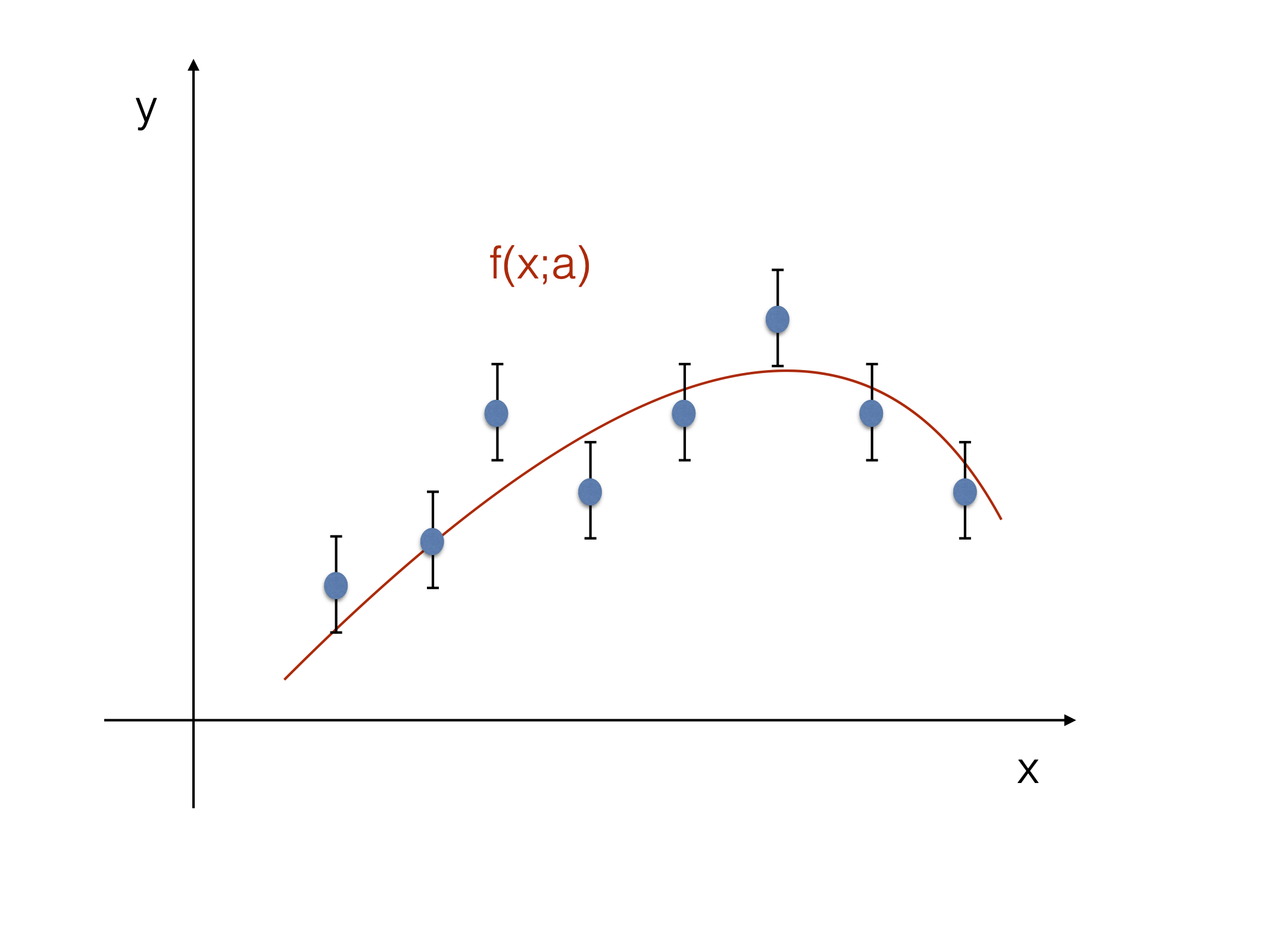
Fig. 16 FIXME: Sketch to illustrate the notation.

If the data \(\{y_i\}\) are Gaussian distributed around the mean \(f(x_i;a)\) then the sum:

(8)\[\chi^{2} = \sum_{i=1}^{N}\left(\frac{y_{i} -f(x_{i};a)}{\sigma_{i}} \right)^{2}\]

obeys a \(\chi^{2}\)-distribution with \((N-1)\) degrees of freedom (the number of measurements, minus the number of fitted parameters). In the general case of \(p\)-parameters to be fitted (\(f(x_i;a)\to f(x_i;\vec{a})\) ) the number of degrees of freedom will be \(N-p\).

To find the best estimate for the parameter \(a\) we proceed in a way similar to what we have done in the ML-method: we look for the value of the parameter \(a\) which minimize the \(\chi^2\). If you interpret the \(\chi^2\) as a distance, the LS method corresponds to minimize the distance between the measured data and the considered model. This boils down to calculating the minimum of the \(\chi^2\) as:

\[ \frac{d\chi^2}{da} = 2 \sum_{i=1}^N \frac{d}{da}f(x_i;a) \cdot \frac{y_i - f(x_i ; a)}{\sigma_i^2} = 0. \]

In case of \(p\) parameters \(a_1,\ldots,a_p\) and \(f(x;\vec{a})\), the idea is the same, just the minimization will have to be performed simultaneously in \(p\) dimensions.

Connection to the Likelihood Function

The simplest way to see the relation between the LS and the ML methods is to take a set of data \((x_{i},y_{i})\) for which the \(x_{i}\) are known precisely and the \(y_{i}\) are known with uncertainties \(\sigma_{i}\). Under the assumption that the \(y_{i}\) are Gaussian distributed (for instance when coming from the CLT), the probability to observe \(y_i\) given the prediction \(f(x_i;a)\) is:

\[ p(y_i|a)=\frac{1}{\sigma_i\sqrt{2\pi}}e^{-(y_i-f(x_i|a))^2/2\sigma_i^2} \]

From this we can build the likelihood function for the complete data set as:

\[\begin{split} \begin{aligned} L(a,\vec{y})&=&\prod_ip(y_i|a) \\ \ln L(a,\vec{y})&=&-\frac{1}{2}\sum_{i} \left(\frac{y_i-f(x_i|a)}{\sigma_i}\right)^2 -\sum_{i} \ln\sigma_i\sqrt{2\pi},\end{aligned} \end{split}\]

where only the first term depends on \(a\). To minimize the negative log-likelihood as a function of the parameter \(a\) we will have to minimize:

\[ \chi^2=\sum_{i} \left(\frac{y_i-f(x_i|a)}{\sigma_i}\right)^2 \]

which corresponds to the \(\chi^2\) procedure shown in the previous section.

Fitting a Straight Line

As a first example of the application of the LS method, we take a set of \(N\) independent measurements \((x_i,y_i)\) where we assume that the model is linear, and in particular that \(f(x) = mx\) (i.e. a straight line passing through the origin). The quantity which has to be minimized is then:

\[ \label{} \chi^2=\sum_i\left(\frac{y_i-mx_i}{\sigma_i}\right)^2 \]

We furthermore assume that all the uncertainties are the same: \(\sigma_{i} = \sigma \, \, \forall i\). Differentiating with respect to \(m\) and equating to zero to obtain the best estimator \(\hat{m}\), we have:

\[\begin{split}\begin{aligned} \frac{\partial \chi^2}{\partial m}&=&-\frac{2}{\sigma^2}\sum_i(x_iy_i-mx_i^2)\\ \sum_i(x_iy_i-mx_i^2) &=&0 \\ \sum_i x_iy_i&=&m\sum_i x_i^2 \\ \hat{m}&=&\sum_i\frac{x_i y_i}{N\overline{x^2}}=\frac{\overline{xy}}{\overline{x^2}} \qquad \left(\sum x_i^2 = N \overline{x^2}\right)\end{aligned} \end{split}\]

The variance of \(\hat{m}\) can be determined by error propagation to be:

\[ V(\hat{m})=\sum_i\left(\frac{x_i}{N\overline{x^2}}\right)^2\sigma^2=\frac{\sigma^2}{N\overline{x^2}}. \]

When the straight line does not pass through the origin, \(f(x_{i};m,b) = mx_{i} + b\) the solution of the LS method is:

(9)\[\begin{split}\begin{aligned} \hat{m} &=& \frac{\overline{xy}-\bar{x}\bar{y}}{\overline{x^2}-\bar{x}^2} \\ \hat{b} &=& \bar{y}-\hat{m}\bar{x} \end{aligned}\end{split}\]

The variances are given by:

\[\begin{split}\begin{aligned} \sigma_m^2 &=& V(\hat{m})=\frac{\sigma^2}{N(\overline{x^2}-\bar{x}^2)} \\ \sigma_b^2 &=& V(\hat{b})=\frac{\sigma^2\overline{x^2}}{N(\overline{x^2}-\bar{x}^2)} \\ cov(\hat{m},\hat{b}) &=& -\frac{\sigma^2\bar{x}}{N(\overline{x^2}-\bar{x}^2)} \\\end{aligned} \end{split}\]

The \(\chi^{2}\) for the best fit is:

\[ \chi^2 =\frac{V(y)}{\sigma^2}(1-\rho^2(x,y)) \]

Note that \(V(y)\) is not the same as \(\sigma^{2}\)!

\(V(y) = \bar{y^{2}} - \bar{y}^{2}\) is the variance of the whole data sample, whereas \(\sigma\) describes the standard deviation of a single measurement around its true value (here we assumed \(\sigma_i = \sigma \; \forall i\)).

If the errors \(\sigma_{i}\) are not all the same, we have to minimize the following expression:

\[ \sum_i\frac{(y_i-mx_i-b)^2}{\sigma_i^2}. \]

The solution of this minimization can again be obtained by the equations given above, if the two means \(\bar{x}\) and \(\bar{y}\) are replaced by the weighted means. Furthermore the normalization is no longer given simply given by \(N\) but it is given by \(\sum_{i} 1/\sigma_{i}^{2}\):

\[ \frac{\sum_i y_i}{N}\to \frac{\sum_iy_i/\sigma_i^2}{\sum_i 1/\sigma_i^2} \]

And the quantity \(\sigma^{2}\) has to be replaced in the expressions for the variance by

\[ \sigma^2\to \frac{N}{\sum_i 1/\sigma_i^2}. \]

For the sake of completeness we give here the full solution in a form which is particularly useful when plugged into a program. We define:

\[\begin{split} \begin{aligned} S_1&=&\sum_i w_i=\sum_i 1/\sigma_i^2 \\ S_x &=&\sum w_i x_i \quad S_y=\sum_i w_iy_i \\ S_{xx}&=&\sum_iw_ix_i^2 \quad S_{xy}=\sum_iw_ix_iy_i \quad S_{yy}=\sum_iw_iy_i^2\end{aligned} \end{split}\]

With this notation we can rewrite the linear system of equation as

\[\begin{split}\left(\begin{array}{cc} S_1 & S_x \\ S_x & S_{xx} \\ \end{array}\right)\cdot {b \choose m} ={S_y \choose S_{xy}}. \end{split}\]

With the expression of the determinant \(D\): $\( \begin{aligned} D&=&S_1S_{xx}-S_x^2 \\\end{aligned} \)$

we can compute:

\[\begin{split} \begin{aligned} \hat{b}&=&(S_{xx}S_y-S_xS_{xy})/D \\ \hat{m}&=&(-S_{x}S_y+S_1S_{xy})/D\end{aligned} \end{split}\]

Once the slope \(\hat{m}\) and the intercept \(\hat{b}\) are obtained, we can compute the uncertainty for an arbitrary interpolated (or extrapolated) point \(y\) for a given \(x\). For such a given \(x\) the predicted value for \(y\) is just \(y = \hat{m} x + \hat{b}\) and the error for the interpolated value \(y\) is then:

\[\begin{split} \begin{aligned} V(y)&=&V(\hat{m}x+\hat{b})=V(\hat{m}x)+V(\hat{b})+2\cdot cov(\hat{m}x,\hat{b})\\ V(y)&=&x^2V(\hat{m})+V(\hat{b})+2x\cdot cov(\hat{m},\hat{b}) \\ V(y)&=&\frac{\sigma^2(x-\bar{x})^2}{N(\overline{x^2}-\bar{x}^2)}+\sigma^2/N\end{aligned} \end{split}\]

We will see in Ch. MVA how this will be used as a simple learning algorithm.

Considering the systematic Errors

As an example we consider a straight line fit where all the measurements \(y_{i}\) have a common statistic error \(\sigma\) and a common systematic error \(S\). We know from the discussion about systematic errors in Ch. Uncertainties that the covariance matrix \(cov(y_{i},y_{j})\) can be written as \(cov(y_{i},y_{j}) = \delta_{ij}\sigma^{2} +S^{2}\). The estimators for the slope and the intercept, \(\hat{m}\) and \(\hat{b}\), respectively, are again given by (9).

The complete formula for the variances reads therefore as follows:

(10)\[\begin{split}\begin{aligned} V(\hat{m})&=&\frac{1}{N^2(\overline{x^2}-\bar{x}^2)^2}\sum_{i,j}(x_i-\bar{x})(x_j-\bar{x})\cdot cov(y_i,y_j) \\ &=&\frac{1}{N^2(\overline{x^2}-\bar{x}^2)^2}\left(\sum_i(x_i-\bar{x})^2\sigma^2+ \sum_{i,j}(x_i-\bar{x})(x_j-\bar{x})S^2\right)\\ &=&\frac{1}{N^2(\overline{x^2}-\bar{x}^2)^2}\left(\sum_i(x_i-\bar{x})^2\sigma^2\right) \end{aligned}\end{split}\]

The second summand in Eq. (10) vanishes, because \(1/N \sum x_{i} = \bar{x}\).

The variance for \(\hat{b}\) is:

\[ V(\hat{b})=\frac{1}{N^2(\overline{x^2}-\bar{x}^2)^2}\sum_{i,j}(\overline{x^2}-\bar{x}x_i) (\overline{x^2}-\bar{x}x_j)\cdot cov(y_i,y_j) \]

The sum \(\sum_i (\overline{x^2}-\bar{x}x_i)=N(\overline{x^2}-\bar{x}^2)\) does not vanish in this equation, thus an additional term appears which is just \(S^{2}\); a common systematic error only influences the variance of the intercept, but it does not change the variance of the slope, as we would have naively expected.

Straight Line Fit with Errors on both Variables

Now we allow for both variables \(x_{i}\) and \(y_{i}\) to have errors \(\sigma_{x_{i}}\) and \(\sigma_{y_{i}}\) (see Fig. 17 and Fig. 18). This means that the sum of the squared residuals of the error ellipsis of the straight line has to be minimized, i.e.:

\[ S(m,b)=\sum_i\frac{(y_i-mx_i-b)^2}{\sigma^2_{y_i}+m^2\sigma^2_{x_i}} \]

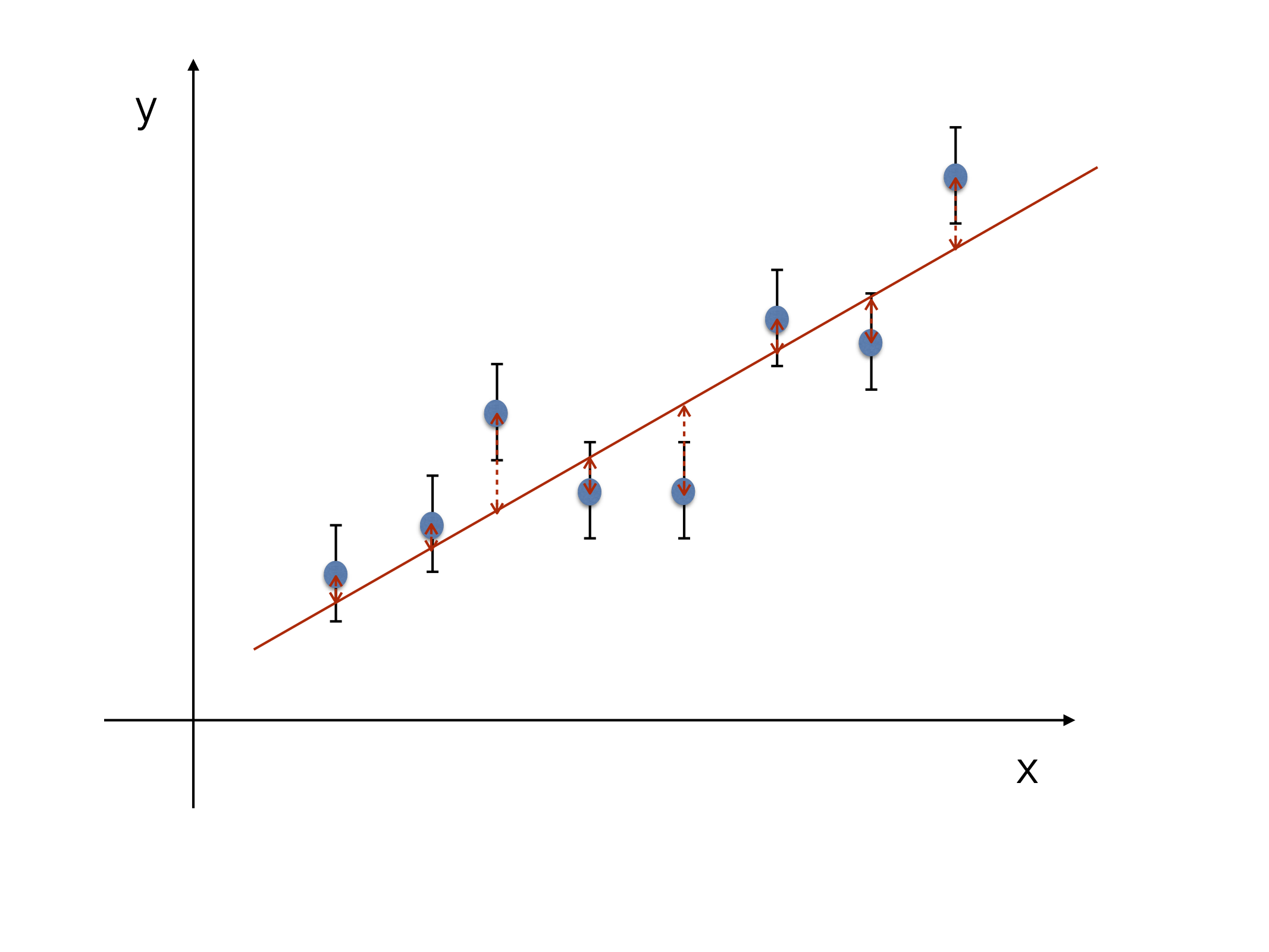
Fig. 17 LS fit with uncertainty only on “y”

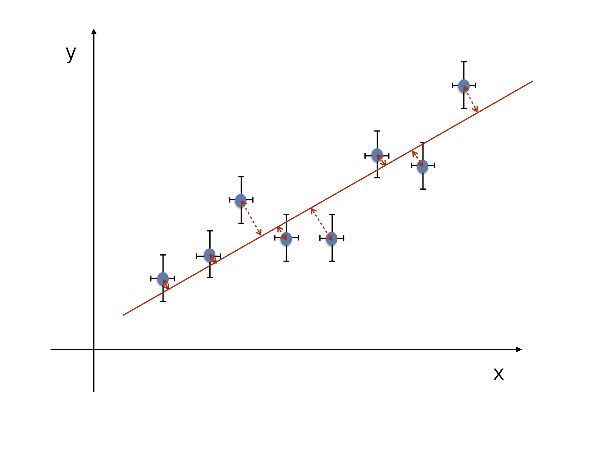
Fig. 18 LS fit with uncertainty on both “x” and “y”.

As usual, the two equations \(\partial S / \partial m = 0\) and \(\partial S / \partial b = 0\) have to be solved.
The condition \(\partial S / \partial b = 0\) leads to

\[ \hat{b}=\frac{\sum y_i/\kappa_i-\hat{m}\sum x_i/\kappa_i}{\sum 1/\kappa_i} \]

where \(\kappa_i=\sigma^2_{y_i}+m^2\sigma^2_{x_i}\). For \(\hat{m}\), if the errors are all the same on \(x\) (i.e. \(\sigma_{x_{i}} = \sigma_{x}\)) and on \(y\) (i.e. \(\sigma_{y_{i}} = \sigma_{y}\)), then the solution for the straight line fit is given by:

\[\begin{split} \begin{aligned} \hat{m}&=&\frac{\sigma_x}{\sigma_y}(A\pm\sqrt{A^2+1}) \\ A&=&\frac{\sigma_x^2V(y)-\sigma_y^2V(x)}{2\sigma_x\sigma_y\cdot cov(x,y)} \\ \bar{y}&=&\hat{m}\bar{x}+\hat{b} \end{aligned} \end{split}\]

Other particular cases can be found making assumption on the uncertainties, but to solve the generic problem numerical techniques are typically used.

Matrix Notation and the uncertainty on the fitted parameters

Let \({\bf a}\) be a vector of \(n\) parameters \(\{a_{i}\}, i=1,\ldots,n\). The \(N\) measured data points can be represented by a vector \({\bf y} = \{y_{i}\},~ i=1,\ldots,N\) and the function to be fitted as \(f(x_{i};{\bf a})\). The \(\chi^2\) expression in matrix form becomes:

\[\begin{split} \begin{aligned} \chi^2&=&\sum_i\sum_j[y_i-f(x_i;{\bf a})]V_{ij}^{-1}[y_j-f(x_j;{\bf a})]\\ &=&({\bf y}-{\bf f})^T{\bf V}^{-1}({\bf y}-{\bf f})={\bf r^T}{\bf V}^{-1}{\bf r} \end{aligned} \end{split}\]

Here, \({\bf r} = {\bf y} - {\bf f}\) is the vector of residuals and \(\bf{V}\) is the covariance matrix. By differentiating \(\chi^{2}\) w.r.t each \(a_{i}\) and equating each of them to zero yields \(n\) equations, which have to be solved simultaneously in order to get the estimator \({\bf \hat{a}}\). Many mathematical packages (e.g. MatLab, Octave, etc…) offer a way to solve matrix problems; in slang moving from the single components equations to the matrix form is called “vectorization”. Because they use highly optimized algorithms, it is always preferable to work with the vectorized version of the problem.

Let \(f(x;{\bf a})\) be a linear function of the parameters \({\bf a}\): \(f(x;{\bf a})=\sum_r c_r(x) a_r\). Where the linearity is on the \({\bf a}\), the \(c_r(x)\) can be any function of \(x\). Written in matrix form, it reads:

\[ \chi^2=({\bf y}-{\bf Ca})^T{\bf V}^{-1}({\bf y}-{\bf Ca}). \]

If we have \(N\) data points and \(n\) coefficients \((n \le N)\), then \({\bf y}\) and \({\bf a}\) are column vectors with dimension \(N\) and \(n\), respectively. The covariance matrix \({\bf V}\) has dimension \(N \times N\) and the matrix \({\bf C}\) has dimensions \(N \times n\).

Minimizing the \(\chi^2\), the equations \(\partial \chi^{2} / \partial {\bf a} = 0\) are:

\[ \partial \chi^{2} / \partial {\bf a} = -2 ( \bf{C}^T \bf{V}^{-1} {\bf \bf{y}} - \bf{C}^T \bf{V}^{-1}\bf{C} {\bf a}) = 0 \]

The solution for the estimator \(\hat{ {\bf a}}\) is then:

\[ {\bf \hat{a}}=({\bf C^T}{\bf V}^{-1}{\bf C})^{-1}{\bf C^T}{\bf V}^{-1}{\bf y} := \bf{B}{\bf y} \]

which means that the solution \({\bf a}\) are linear functions of the measurements \({\bf y}\).

Using error propagation we can find the covariance matrix for the \({\bf \hat{a}}\):

\[ \bf{U} = \bf{B} \bf{V} \bf{B}^T = [{\bf C^TV}^{-1}{\bf C}]^{-1} \]

Example:

Let’s go back to the fit of a straight line of the form \(f(x) = mx + b\) to \(N\) data points, which have independent and common errors, such that \({\bf V} = \sigma^{2} I\), i.e. \(V_{ij} = \sigma^{2} \delta_{ij}\). In matrix notation we then get:

\[\begin{split} \begin{array}{cc} f_1 & = b+ mx_1 \\ f_2 & = b+ mx_2 \\ \vdots & \vdots \\ f_N & = b+ mx_N \\ \end{array} \qquad {\bf C} = \left( \begin{array}{cc} 1 & x_1 \\ 1 & x_2 \\ \vdots & \vdots \\ 1 & x_N \\ \end{array} \right) \end{split}\]

\[ {\bf \hat{a}} = \sigma^2({\bf C^TC})^{-1}\frac{1}{\sigma^2}{\bf C^Ty} \]

which can be explicitly written as:

\[\begin{split} \label{matrix_ls} {\bf \hat{a}}=\left(\begin{array}{c} \hat{b} \\ \hat{m} \end{array} \right) = \left(\begin{array}{cc} \sum_i 1 & \sum_i x_i \\ \sum_i x_i & \sum_i x_i^2 \\ \end{array} \right)^{-1} \left(\begin{array}{c} \sum_i y_i \\ \sum_i x_iy_i \end{array} \right) \end{split}\]

The inversion of the \(2 \times 2\)-matrix gives:

\[\begin{split} \frac{1}{N(\overline{x^2}-\bar{x}^2)} \left(\begin{array}{cc} \overline{x^2}& -\bar{x} \\ -\bar{x} & 1 \\ \end{array} \right) \end{split}\]

which finally leads to:

\[\begin{split} {\bf \hat{a}}=\left(\begin{array}{c} \hat{b} \\ \hat{m} \end{array} \right) = \frac{1}{N(\overline{x^2}-\bar{x}^2)} \left(\begin{array}{cc} \overline{x^2}& -\bar{x} \\ -\bar{x} & 1 \\ \end{array} \right) \left(\begin{array}{c} \sum_i y_i \\ \sum_i x_iy_i \end{array} \right). \end{split}\]

Which corresponds to the expressions for \(\hat{m}\) and \(\hat{b}\) which we extracted in (9).

The variance for the estimator \(\hat{ {\bf a}}\) is:

\[\begin{split} {\bf V}({\bf\hat{a}})=\left(\begin{array}{cc} V(b)& cov(b,m) \\ cov(b,m) & V(m) \\ \end{array} \right) = \frac{\sigma^2}{N(\overline{x^2}-\bar{x}^2)}\left(\begin{array}{cc} \overline{x^2}& -\bar{x} \\ -\bar{x} & 1 \\ \end{array} \right) \end{split}\]

Example:

In a second example we fit the parabola \(f(x) = a_{0} + a_{1} x + a_{2} x^{2}\) to \(N\) data points. Again we assume the errors being independent and equal for all data points. The matrix \({\bf C}\) is now given by:

\[\begin{split} {\bf C}=\left( \begin{array}{ccc} 1 & x_1 & x_1^2\\ 1 & x_2 & x_2^2\\ \vdots & \vdots & \vdots \\ 1 & x_N & x_N^2 \\ \end{array} \right) \end{split}\]

Going through the same steps as for the linear case we obtain:

\[\begin{split} {\bf \hat{a}}= \left( \begin{array}{c} \hat{a_0} \\ \hat{a_1} \\ \hat{a_2}\\ \end{array} \right) =\left( \begin{array}{ccc} \sum_i 1 & \sum_i x_i & \sum_i x_i^2 \\ \sum_i x_i & \sum x_i^2 & \sum_i x_i^3 \\ \sum_i x_i^2 & \sum x_i^3 & \sum_i x_i^4 \\ \end{array} \right)^{-1} \left( \begin{array}{c} \sum_i y_i \\ \sum_i x_iy_i \\ \sum x_i^2y_i\\ \end{array} \right) \end{split}\]

The generalization of this method to higher-order polynomials follows the same pattern.

Another way to write the (inverse) of the covariance matrix is:

\[ (U^{-1})_{ij} = \frac{1}{2}\left[ \frac{\partial^2 \chi^2}{\partial a_i \partial a_j } \right]_{\bf a = \hat{a}} \]

which is the expression of the RCF bound in the case that the measurements \({\bf y}\) are Gaussian distributed, and where we use the relation with the log likelihood \(- \ln L = \chi^2/2\) (a part from an overall constant).

Again in case of a function \(f\) linear in \({\bf a}\), the \(\chi^{2}\) becomes quadratic in \({\bf a}\):

\[ \chi^2({\bf a})=\chi^2({\bf \hat{a}})+\frac{1}{2}\sum_{i,j=1}\left[\frac{\partial^2\chi^2}{\partial a_i\partial a_j}\right]_{a=\hat{a}}(a_i-\hat{a}_i)(a_j-\hat{a}_j) \]

Using the expression of the variance we just found, the equation above corresponds to contours in the parameter space defined by \(\hat{a}_i\pm \hat{\sigma_i}\) and therefore giving the \(\pm 1 \sigma\) deviations from the estimators:

\[ \chi^2({\bf a}\pm \hat{\sigma})=\chi^2({\bf \hat{a}})+1=\chi^2_{min}+1. \]

Hence the \(\chi^{2}\)-function is a parabola with a minimum at \(\hat{a}\) and the errors \(\sigma\) for the estimators are determined by \(\chi^{2}_{min}+1\). In general, if the function \(f\) is not linear in the parameters, the contour will not be an ellipse, but it will still define a confidence region reflecting the statistical uncertainty on the fitted parameters. The precise construction of the confidence region will be developed in Sec. Confidence Limits. It is important to notice that the confidence level of the region defined by the contour, depends on the number of parameters fitted: 6.83% for one parameter, 39.4% for two, 19.9% for three, etc… (see again Sec. Confidence Limits).

Binned \(\chi^{2}\) fit

In this section we will apply the LS method to binned data. In the case of \(f\) being a probability distribution function (a p.d.f. instead of any generic function), we can interpret the value of \(f\) integrated over a given range (“bin”), as the expected number of events in that bin \(f_i = E[y_i]\): $\( \label{eq:LS} f_i({\bf a}) = n\int_{x_i^{min}}^{x_i^{max}} f(x;{\bf a}) dx = n p_i({\bf a}) \)$

where \(x_i^{min}\) and \(x_i^{max}\) are the bin boundaries, the \(p_i({\bf a})\) is the probability to have an event in the bin \(i\), given the parameters \({\bf a}\) and n is the overall normalization.
The fit proceeds as before minimizing the \(\chi^2\) w.r.t. the parameters \({\bf a}\):

\[ \chi^2(y_i|{\bf a})=\sum_i \frac{(y_i - f_i({\bf a}))^2}{\sigma_i^2} \]

where here \(\sigma_i\) is the variance of the expected number of entries in bin \(i\). If the number of entries in bin \(i\) is small compared to the total number of entries in the histogram then we can assume that they are Poisson distributed and the variance is equal to the mean \(\sigma_i^2 = f_i({\bf a}) = n p_i({\bf a})\).
Often, instead of using the variance of the expected number of entries in bin \(i\), the variance of the observed number of entries in bin \(i\) is used, leading to:

\[ \chi^2(y_i|{\bf a})=\sum_i \frac{(y_i - f_i({\bf a}))^2}{y_i}. \]

This new expression is called the modified LS method. Even if computationally easier to implement (contraty to \(\sigma_i^2\) the observed \(y_i\), obviously, does not depend on \(\bf{a}\)), it brings in the problem of the variance estimation for bins which are poorly populated or have no entries at all. As a rule of thumb, try to have at least 5 entries per bin. Two situations are rather typical: small statistics in the tails of a distribution, or the whole histogram is sparsely populated. In the first case, try to rebin, for the latter just move to an unbinned ML fit to use the full information you have in your data.

Use of the \(\chi^2\) to test the goodness of fit

If the \(\chi^{2}\) is large after minimization, then the function is probably badly chosen (i.e. not correctly describing the data); intuitively, the \(\chi^{2}\) should be small if the function describes the data. On the other hand, the \(\chi^{2}\) can be small if you have too many degrees of freedom (fit n-points with a polynomial of degree n) or, even with a bad model, when the uncertainties are overestimated (\(\sigma_i^2\) sits at the denominator). You can always get very small \(\chi^{2}\) if you assume large enough uncertainties! If the errors are too large the whole method loses its predictive power.

We have already encountered in Chi2 distribution the \(\chi^{2}\)-distribution:

\[ f(\chi^2;n)=\frac{2^{-n/2}}{\Gamma(n/2)}\chi^{n-2}e^{-\chi^2/2}. \]

The distribution depends on \(n\), the number of degrees of freedom, which is the number of data points minus the number of parameters of the model. Because the \(\chi^{2}\) distribution has expectation value \(n\) and variance \(2n\), we expect the \(\chi^{2}\) divided by the number of degrees of freedom to be approximately one: \(\chi^{2} / n \approx 1\). If the \(\chi^{2} / n\) is much larger than one, the data are not properly described by the model. Let’s introduce the definition of \(p-\)value to quantify the level of agreement of the model with data:

(11)\[p=\int_{\chi^2}^\infty f(x';n) dx' \]

where \(f(x';n)\) is the \(\chi^2\) distribution for \(n\) degrees of freedom. Values can be computed in FIXME ROOT using TMath::ChisquareQuantile(Double_t p, Double_t ndf).

The \(p-\)value for a given \((\chi^2; n)\) is a measurement of the “goodness of fit”; when repeating the experiment several times it gives the probability, under the hypothesis \(f\), of obtaining a result as incompatible with \(f\) or worse (i.e. \(\chi^2\) equal or larger) than the one actually observed. The threshold on the \(p-\)value used to reject the model is subjective; typical values used are of a few percent. Fig. 19. maps the relation between the \(\chi^2\), the number of degrees of freedom and the \(p-\)value. In particular is shown the example where, for \(n=4\), a \(\chi^2>6\) will be observed in 20% of the cases.

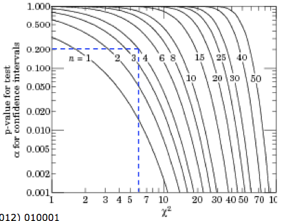
Fig. 19 One minus the \(\chi^2\) cumulative distribution, \(1 - F (\chi^2; n)\), for n degrees of freedom. This gives the \(p-\)value for the \(\chi^2\) goodness-of-fit test.

We will come back in Hypothesis Testing to different quantitative ways to evaluate the compatibility of the data with a model

References

Most of the material of this section is taken from:

• G. Cowan, [Cow98], “Statistical Data Analysis”,Ch. 7