Probability Distributions#
In this chapter, we will review key concepts in combinatorics and then introduce the most common probability distributions in physics, including discrete distributions (probability mass functions) and continuous distributions (probability density functions). We will conclude the chapter with one of the most important theorems in statistics: the Central Limit Theorem.
Basic combinatorics#
Let’s start with some nomenclature and some basic results from combinatorics that will be needed for what follows.
In this section we will be talking about sequences of objects: a distinction has to be made on whether we care or not about the order of the elements in a sequence. If we care about the order we talk about permutations, otherwise we talk about combinations (permutations are ordered combinations).
Example:
take the set of letters \(\{abc\}\). The sequences \(\{cab\}\) and \(\{bac\}\) are considered equivalent combinations but distinct permutations.
Factorial#
The number of ways to order a set of n distinct objects is given by the factorial:
n!=n×(n−1)×(n−2)×⋯×2×1
This accounts for every possible arrangement (permutation) of the n objects.
For large \(n\), the Stirling formula can be used to approximate \(n!\):
The factorial \(n!\) can be extended for non-integer arguments \(x\) by the gamma function \(\Gamma(x)\):
Permutations with repetitions:#
pick r objects from a set of n and put them back each time. The number of permutations (ordered sequences) is:
\(n^r\)
Example:
A byte is a sequence of 8 bits (0/1): the number of permutations with repetitions is \(2^8 = 256\). A lock with three digits (form 0 to 9) has \(10^3\) permutations.
Permutations without repetitions:#
pick r objects from a set of n and don’t put them back. At each pick you will have one less object to choose from, so the number number of permutations is reduced with respect to \(n^r\) (permutations with repetitions). The number of permutations (ordered sequences) is:
\(\frac{n!}{(n-r)!}\)
Example:
take all permutations without repetitions of the 52 cards in the deck: 52! (first pick you choose among 52 cards, second pick among 51 etc…). Take all permutations of the first 4 picks in a deck of 52 cards: \(52\cdot51\cdot50\cdot49 = 52!/ (52-4)!\) (first you pick from 52, then from 51, then from 50, then form 49).
Combinations without repetitions:#
pick r objects from a set of n and don’t put them back. At each pick you will have less objects to choose from as for permutations, but this time all sequences that differ only by their order are considered to be the same. The number of combinations (non-ordered sequences) is the number of permutations corrected by the factor that describes the number of ordered sequences (i.e. r!):
\(\frac{n!}{(n-r)!}\frac{1}{r!} = \binom{n}{r}\)
we read this “n pick r”.
These numbers are the so-called binomial coefficients, which appear in the binomial theorem:
\((p+q)^n=\sum_{r=0}^{n}{n\choose r}\, p^r\cdot q^{n-r}\)
An interesting propertiy is that the number of combinations extracting r objects from n or (n-r) from n is the same.
Example:
“lotto” (six-numbers lottery game): 6 numbers are extracted (without putting them back) from a set of 90. The order of the extraction is irrelevant. The probability to win (when all tickets are sold) is \(1/\binom{90}{6}\) =1.6 \(10^{-9}\).
Combinations with repetitions:#
pick r objects from a set of n and put them back. As in the case of permutations with repetition but this time without considering the order.
\(\frac{(n+r-1)!}{(n-1)!r!} = \binom{n+r-1}{r}\)
Example:
take r-scoops from n-icecream flavours. You can take them all the same or repeat them as you like (assuming there is enough icecream…).
Derivation:
Start from an example: take 3 objects from a set of 5 (a,b,c,d,e).
Examples of those sequences are (a a b),\(\;\) (a b c),\(\;\) (c c c).
Now think about the sequences as ordered boxes filled with the letters:
one box for the a’s, one box for the b’s, etc… I will use a separator
“\(|\)” instead of drawing boxes (this trick will become very important in
a second):
(a a b) \(\rightarrow\) a a \(|\) b \(|\) \(\;\) \(|\) \(\;\) \(|\) (the last three
are empty boxes corresponding to c, d, e)
(a b c) \(\rightarrow\) a \(|\) b \(|\) c \(|\) \(\;\) \(|\) \(\;\)
(c c c) \(\rightarrow\) \(\;\)\(|\) \(\;\) \(|\) c c c \(|\) \(\;\) \(|\)
We can also drop the letters and replace them with “x”, the position of
the box already tells which letter it correspnds to.
e.g.: aab \(\rightarrow\) a a \(|\) b \(|\) \(\;\) \(|\) \(\;\) \(|\) \(\rightarrow\) x
x \(|\) x \(|\) \(\;\) \(|\) \(\;\) \(|\)
Considering “x” and “\(|\)” as objects (here is where the trick becomes
important), we can rephrase the problem as “in how many ways we can
place r = 3 “x” and n = 5-1 = 4 “\(|\)”.
This is the same as the combination w/o repetition “N pick R”, where in
this case:
N = n-1 + r (sum of all “\(|\)” and “x”) R = r \(\;\;\;\;\;\Rightarrow\binom{n-1+r}{r}\)
Discrete Distributions#
Bernoulli trials#
A Bernoulli trial is an experiment with only two outcomes (success/failure or 1/0) and where success will occur with constant probability \(p\) and failure with constant probability \(q=1-p\). Examples are again the coin toss, or (from particle physics) the decay of \(K^{+}\) into either \(\mu^{+}\nu\) or any other channels. The random variable \(r\in\{0,1\}\) is the outcome of the experiment and its p.d.f. is:
The p.d.f. is simply the probability for a single experiment to give success/failure. The first two moments of the distribution are:
The distribution for a given value of p is:

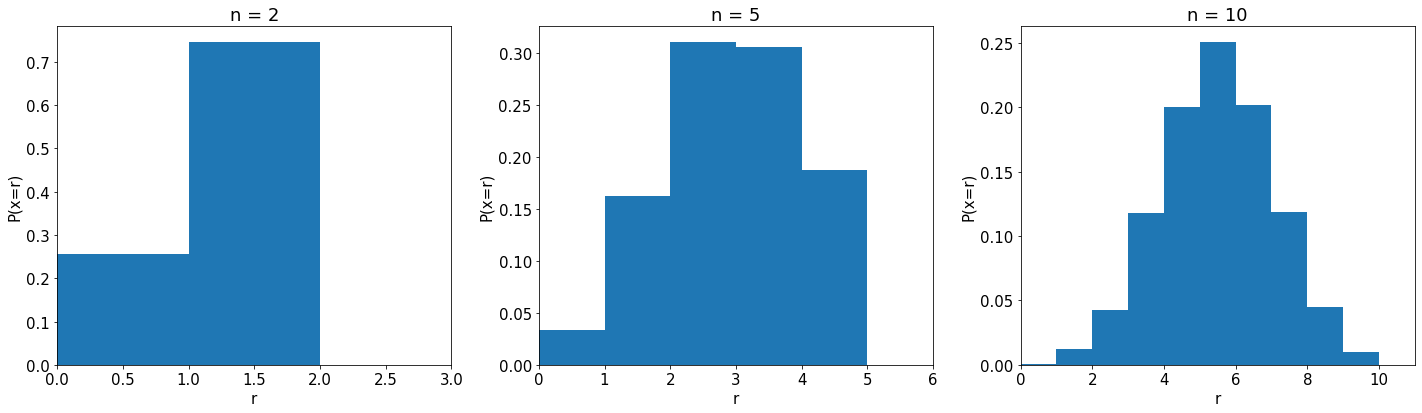
Binomial#
Given \(n\) Bernoulli trials with a probability of success \(p\), the binomial distribution gives the probability to observe \(r\) successes and, consequently, \(n-r\) failures independently of the order with which they appear. The random variable is again \(r\) but this time \(r\in\{0,n\}\), i.e. the maximum is given when all trials give a success. The p.d.f. is:
Eq.(2) can be motivated in the following way: the probability that we get a positive outcome in the first \(r\) attempts and negative outcome in the last \(n-r\) attempts, is given by \(p^{r} \cdot (1-p)^{n-r}\); but this sequential arrangement is only one of a total of \({n \choose r}\) possible arrangements. The distribution for different values of the parameters is plotted below.
The important properties of the binomial distribution are:
It is normalized to 1, i.e. \(\sum_{r=0}^n P(r)=1.\)
The mean of \(r\) is \(<r>=\sum_{r=0}^n r\cdot P(r)=np.\)
The variance of \(r\) is \(V(r)=np(1-p).\)
The binomial distribution (like several others we will encounter) has the reproductive property:
if \(X\) is binomially distributed as \(P(X;n,p)\) and \(Y\) is binomially distributed (with the same probability \(p\)) as \(P(Y;m,p)\), then the sum is binomially distributed as \(P(X+Y; n+m, p)\).
Example:
What is the probability to get out of 10 coin tosses 3 times a “head”? Solution: \(P(3; 10, 0.5)={10 \choose 3}\,0.5^3\cdot (1-0.5)^{10-3}=\frac{10!}{3!7!}0.5^3\cdot 0.5^7=0.12\)
Example:
A detector with 4 layers has an efficiency per layer to create a hit from a traversing particle of 99%.
What is the probability to reconstruct a tracklet with 2 or 3 or 4 hits ? and what is the probability to reconstruct a tracklet with at least 2 hits ?
P(r = 2; n = 4, p=0.99) = 0.00 (0.0006)
P(r = 3; n = 4, p=0.99) = 0.038
P(r = 4; n = 4, p=0.99) = 0.96
P(r ≥ 2; n = 4, p=0.99) = sum of the above > 99%
Multinomial Distribution#
The precedent considerations can directly be generalized in this way: assume we have \(n\) objects of \(k\) different types, and \(r_{i}\) is the number of objects of type \(i\). The number of distinguishable arrangements is then given by \(\frac{n!}{r_1!r_2!\cdots r_k!}\). If we now choose randomly
objects (putting them back every time), then the probability of getting an arrangement of \(r_{1}\) objects of type \(1\), \(r_{2}\) objects of type \(2\), etc… is given by \(p_1^{r_1}\cdot p_2^{r_2}\cdots p_k^{r_k}\). The overall probability is therefore simply the probability of our arrangement, multiplied with the number of possible distinguishable arrangements:
This distribution is called the multinomial distribution and it is what describes the probability to have \(r_i\) events in bin i of a histogram with \(n\) entries. The corresponding properties are:
You can also compute the covariance among the bins of a histogram:
and the correlation coefficient:
The correlation among bins comes from the fact that the total number of entries \(n = r_1+\ldots+r_k\) is fixed, i.e. \(r_i = n - r_1 - \ldots - r_{i-1} - r_{i+1} -\ldots - r_k .\)
If n is not fixed, i.e. n is another random variable, the bin entries are uncorrelated and instead of having a multinomial we will have a Poisson for each bin (see also extended maximum likelihood fit).
import numpy as np
import matplotlib.pyplot as plt

# Define parameters
n = 100  # Total number of trials
p = [0.1, 0.2, 0.5, 0.1, 0.1]  # Given probability distribution

# Generate a random sample from a multinomial distribution
observed_counts = np.random.multinomial(n, p)

# Compute expected counts
expected_counts = np.array(p) * n

# Compute error bars for observed counts (using Poisson statistics)
errors = np.sqrt(observed_counts)  # Poisson uncertainty ~ sqrt(N)

# Labels for bins
labels = ["Bin 1", "Bin 2", "Bin 3", "Bin 4", "Bin 5"]
x = np.arange(len(labels))

# Plot expected counts as blue bars
plt.bar(x, expected_counts, width=0.6, label="Expected", color="b", alpha=1.0)

# Plot observed counts as black points with error bars
plt.errorbar(x, observed_counts, yerr=errors, fmt='ko', label="Observed", capsize=5)

# Formatting
plt.xticks(x, labels)
plt.ylabel("Counts")
plt.title("Multinomial Distribution")
plt.legend()
plt.show()

print ("Expected: ", expected_counts)
print ("Observed: ", observed_counts)
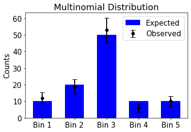
Expected:  [10. 20. 50. 10. 10.]
Observed:  [12 19 53  6 10]
Poisson Distribution#
The Poisson p.d.f. applies to the situations where we detect events, but
do not know the total number of trials. An example is a radioactive
source where we detect the decays but do not detect the non-decays.
The distribution can be obtained as a limit of the binomial: let
\(\lambda\) be the probability to observe a radioactive decay in a period
\(T\) of time. Now divide the period \(T\) in \(n\) time intervals
\(\Delta T = T/n\) small enough that the probability to observe two
decays in an interval is negligible. The probability to observe a decay
in \(\Delta T\) is then \(\lambda / n\), while the probability to observe
\(r\) decays in the period \(T\) is given by the binomial probability to
observe \(r\) events in \(n\) trials each of which has a probability
\(\lambda / n\).
Under the assumption that \(n >> r\) then:
and
we obtain the Poisson p.d.f:
The Poisson distribution can so be seen as the limit of the binomial distribution when the number \(n\) of trials becomes very large and the probability \(p\) for a single event becomes very small, while the product \(pn = \lambda\) remains a (finite) constant. It gives the probability of getting \(r\) events if the expected number (mean) is \(\lambda\).
Properties of the Poisson distribution:
it is normalized to 1: \(\sum_{r=0}^{\infty}P(r)=e^{-\lambda}\sum_{r=0}^{\infty}\frac{\lambda^r}{r!}=e^{-\lambda}e^{+\lambda}=1\)
the mean \(<r>\) is \(\lambda\): \(<r>=\sum_{r=0}^{\infty}r\cdot \frac{e^{-\lambda}\lambda^r}{r!}=\lambda\)
the variance is \(V(r)=\lambda\)
\(P(r+s;\lambda_r, \lambda_s) = \frac{(\lambda_r+\lambda_s)^{(r+s)} e^{-(\lambda_r+\lambda_s)}}{(r+s)!}\): the p.d.f. of the sum of two Poisson distributed random variables is also Poisson with \(\lambda\) equal to the sum of the \(\lambda\)’s of the individual Poissons
Example:
An historical example is the number of deadly horse accidents in the Prussian army. The fatal incidents were registered over twenty years in ten different cavalry corps. There was a total of 122 fatal incidents, and therefore the expectation value per corps per year is given by \(\lambda = 122/200 =0.61\). The probability that no soldier is killed per year and corps is \(P(0;0.61) = e^{-0.61} \cdot 0.61^{0} / 0! = 0.5434\). To get the total events (of no incidents) in one year and per corps, we have to multiply with the number of observed cases (here 200), which yields \(200 \cdot 0.5434 = 108.7\). The total statistics of the Prussian cavalry is summarized in the following table in agreement with the Poisson expectation:
Fatal incidents per corps and year |
Reported incidents |
Poisson distribution |
|---|---|---|
0 |
109 |
108.7 |
1 |
65 |
66.3 |
2 |
22 |
20.2 |
3 |
3 |
4.1 |
4 |
1 |
0.6 |
The Poisson distribution is very often used in counting experiments:
number of particles which are registered by a detector in the time interval \(t\), if the flux \(\Phi\) and the efficiency of the detector are independent of time and the dead time of the detector \(\tau\) is sufficiently small, such that \(\phi \tau \ll 1\)
number of interactions caused by an intense beam of particles which travel through a thin foil
number of entries in a histogram, if the data are taken during a fixed time interval
number of flat tires when traveling a certain distance, if the expectation value flats / distance is constant
Some counter-examples, in which the Poisson distribution cannot be used:
the decay of a small amount of radioactive material in a certain time interval, if this interval is comparable to the lifetime
the number of interactions of a beam of only a few particles which pass through a thick foil
In both cases the event rate is not constant (in the first it decreases with time, in the second with distance) and therefore the Poisson distribution cannot be applied.
The Poisson p.d.f. requires that the events be independent. Consider the case of a counter with a dead time of 1 \(\mu sec\). This means that if a second particle passes through the counter within 1 \(\mu sec\) after one which was recorded, the counter is incapable of recording the second particle. Thus the detection of a particle is not independent of the detection of other particles. If the particle flux is low, the chance of a second particle within the dead time is so small that it can be neglected. However, if the flux is high it cannot be. No matter how high the flux, the counter cannot count more than \(10^6\) particles per second. In high fluxes, the number of particles detected in some time interval will not be Poisson distributed.

Example:
Example of Higgs boson production at the LHC (proton proton collisions):
Remeber the number of expected events is given by the product of the production cross section times the integrated lumiosity: \(N = \sigma \cdot L\).
The probability to produce a Higgs boson following the frequentist definition is: \(p(pp\to H) = \frac{L\sigma(pp\to Higgs)A\epsilon}{L\sigma(pp)}\)
where A and \(\epsilon\) are respectively the acceptance and the efficiency of the analysis.
The Binomial probability to observe \(n_H^{obs}\) events given N collisions and the probability to produce one Higgs boson given above is: \(P(n_H^{obs}) = \binom{N}{n_H^{obs}} p^{n_H^{obs}} (1-p)^{N-n_H^{obs}}\)
Because N is large and p is small we define: \(\lambda = N\cdot p = \sigma(pp) \cdot L \cdot \frac{L\sigma(pp\to Higgs)A\epsilon}{L\sigma(pp)} = n_H^{exp}\)
and approximate the Binomial with a Poisson: \(Poisson(n_H^{obs}, \lambda) = \frac{e^{-\lambda}\lambda^{n_H^{obs}}}{n_H^{obs}!} \)
Continuous Distributions#
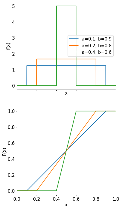
Uniform Distribution#
The probability density function of the uniform distribution in the interval \([a,b]\) is given by:
The expectation value and the variance are given by
\( <x> = \int_a^b\frac{x}{b-a}dx=\frac{1}{2}(a+b) \)
\( \mbox{Var}(x) = \frac{1}{12}(b-a)^2 \)
(This is the source of the \(\sqrt{12}\) when reporting the resolution of a binary detector as the standard deviation of a flat distribution.)
Example:
Consider a detector built as a single strip of silicon with a width of 1mm. If a charged particle hits it, the detector reads 1 otherwise zero (binary readout). What is the spacial resolution of the detector? Estimating the resolution as the root square of the variance of the corresponding uniform distribution, we get \(\sim 290\mu m\).
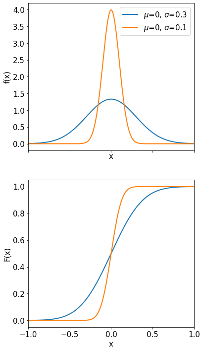
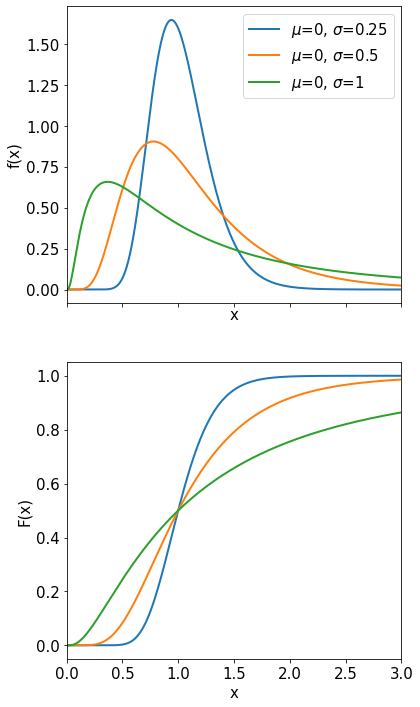
Gaussian or Normal Distribution#
The Gaussian or normal distribution is probably the most important and useful distribution we know. For example it is used to describe your measurements when they are affected by a large number of additive ‘noise’ sources (see CLT later).
The probability density function is
The Gaussian distribution is described by two parameters: the mean value \(\mu\) and the variance \(\sigma^{2}\) or the standard deviation \(\sigma\). By substituting \(z = (x-\mu) / \sigma\) we obtain the so-called normal or standardized Gaussian distribution:
It has an mean of zero and standard deviation 1.
Properties of the normal distribution are:
it is normalized to 1: \(\int_{-\infty}^{+\infty}P(x;\mu,\sigma)dx=1\)
\(\mu\) is the first moment of the distribution: \(\int_{-\infty}^{+\infty}xP(x;\mu,\sigma)dx=\mu\)
being a symmetric distribution, \(\mu\) is also its mode and median
its second central moment is \(\sigma^2\): \(\int_{-\infty}^{+\infty}(x-\mu)^2P(x;\mu,\sigma)dx=\sigma^2\)
If \(X\) and \(Y\) are two independent r.v.’s distributed as \(f(x;\mu_x,\sigma_x)\) and \(f(y;\mu_y,\sigma_y)\) then Z = X + Y is distributed as \(f(z;\mu_z,\sigma_z)\) with \(\mu_z = \mu_x+\mu_y\) and \(\sigma_z^2 = \sigma_x^2 + \sigma_y^2\).
If the two r.v. are not independent you need to add to the sum of variances the term \(\sigma_z^2 = \sigma_x^2 + \sigma_y^2 + cov(X,Y)\).
Careful: here you are summing two random variables ! This means that you are summing one sample from one gaussian to one sample from the second gaussian. You are not summing two gaussian pdfs ! \(f(x) = f_1 G(x | \mu_1, \sigma_1) + (1-f_1)G(x | \mu_2, \sigma_2)\). This is known as a “gaussian mixture model” and in general it is not a gaussian.
Some useful integrals, which are often used when working with the Gaussian function:
Here are some numbers for the integrated Gaussian distribution:
68.27% of the area lies within \(\pm\sigma\) around the mean \(\mu\)
95.45% lies within \(\pm 2\sigma\) around the mean \(\mu\)
99.73% lies within \(\pm 3 \sigma\) around the mean \(\mu\)
90% of the area lies within \(\pm 1.645\sigma\) around the mean \(\mu\)
95% lies within \(\pm 1.960\sigma\) around the mean \(\mu\)
99% lies within \(\pm 2.576\sigma\) around the mean \(\mu\)
99.9% lies within \(\pm 3.290\sigma\) around the mean \(\mu\)
The integrated Gaussian function \(\Phi(x)\) can also be expressed by the so-called error function \(erf(x)\):
The Full Width Half Maximum (FWHM) is very useful to get a quick estimate for the width of a distribution and for the specific case of the Gaussian we have: \(FWHM=2\sigma\sqrt{2\ln 2}=2.355\sigma.\)
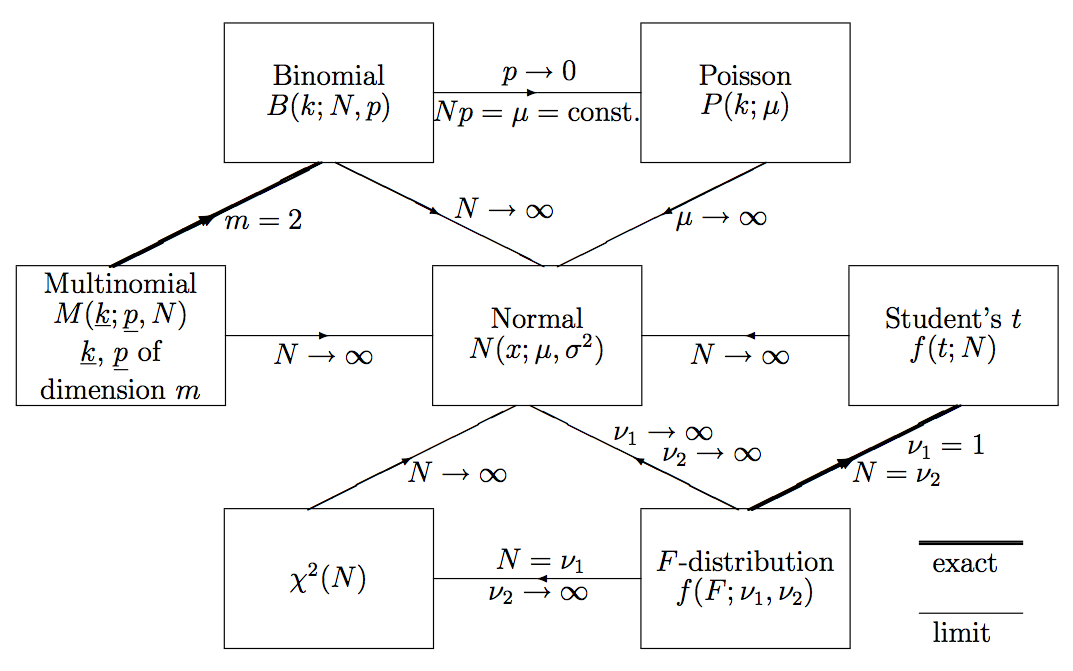
The Gaussian distribution is the limiting case for several other p.d.f.’s we will encounter later (see (see Fig. 3)). This is a consequence of the central limit theorem (CLT) (discussed in CLT)
The N-dimensional Gaussian distribution is defined by
Here, \({\bf x}\) and \({\bf \mu}\) are column vectors with the components \(x_1,\ldots ,x_N\) and \(\mu_1,\ldots ,\mu_N\), respectively. The transposed vectors \({\bf x}^T\) and \({\bf \mu}^T\) are the corresponding row vectors and \(|V|\) is the determinant of the symmetric \(N \times N\) covariance matrix \(V\). The expectation values and the covariances are given by:
\(\langle x_i \rangle=\mu_i\)
\(\mbox{V}(x_i)=\mbox{V}_{ii}\)
\(\mbox{cov}(x_i,x_j)=\mbox{V}_{ij}\)
In the simplified case of a two-dimensional Gaussian distribution we can write
\( \mathbf{x}= \left[ \begin{array}{l} x_1 \\ x_2 \end{array} \right] \) \( \mathbf{\mu }= \left[ \begin{array}{l} \mu_1 \\ \mu_2 \end{array} \right] \) \( V= \left[ \begin{array}{cc} \sigma_1^2 & \rho \sigma_1 \sigma_2 \\ \rho \sigma_1 \sigma_2 & \sigma_2^2 \end{array} \right] \)
where the determinant of V is \(|\boldsymbol{V}|=\sigma_1^2 \sigma_2^2\left(1-\rho^2\right)\).
The inverse of the covariance matrix is: \( V^{-1}=\frac{1}{\sigma_1^2 \sigma_2^2\left(1-\rho^2\right)} \left[ \begin{array}{cc} \sigma_2^2 & -\rho \sigma_1 \sigma_2 \\ -\rho \sigma_1 \sigma_2 & \sigma_1^2 \end{array} \right] \)
So the exponent becomes:
\( ({\bf x}-{\bf \mu})^TV^{-1}({\bf x}-{\bf \mu})= \frac{1}{1-\rho^2}\left[\left(\frac{\left(x_1-\mu_1\right)^2}{\sigma_1^2}\right)-2 \rho\left(\frac{\left(x_1-\mu_1\right)\left(x_2-\mu_2\right)}{\sigma_1 \sigma_2}\right)+\left(\frac{\left(x_2-\mu_2\right)^2}{\sigma_2^2}\right)\right] \)
and putting it all together we have:
We will come back to the specific case of the gaussian distribution in multiple dimensions in the chapter Measurement Uncertainties when talking about the error matrix.
\(\chi^2\) Distribution#
Suppose that \(x_{1}, x_{2}, \cdots, x_{n}\) are independent random variables Normally distributed as N(0,1), then the sum of squares
\( \chi_{(n)}^2=\sum_{i=1}^n x_i^2 \)
is distributed as as a chi-square distribution \(\chi^2(n)\), with n degrees of freedom.
This is generally written as:
You can see why writing the joint p.d.f. of n independent gaussian distributed variables:
and looking at the exponent.
The probability density is given by:
The \(\chi^2(n)\) p.d.f. has the properties:
mean = \(n\)
variance = \(2n\)
mode = n-2 for \(n\ge2\) and 0 for \(n\le2\)
reproductive property: \(\chi^2_{n_1+n_2} = \chi^2_{n_1} + \chi^2_{n_2} = \chi^2(n_1+n_2)\)
Since the expectation of \(\chi^2(n)\) is \(n\), the expectation of \(\chi^2(n)/n\) is 1. The quantity \(\chi^2(n)/n\) is called “reduced \(\chi^2\)”.
For \(n \to \infty\), \(\chi^{2}(n)\to N(\chi^2;n,2n)\) becomes a normal distribution. In practice, the approximation by a normal distribution is already good enough for \(n \ge 30\).
Log-Normal Distribution#
The log-normal distribution is defined as the distribution of a random variable whose logarithm is normally distributed; i.e. if \(y\) obeys a normal distribution with mean \(\mu\) and standard deviation \(\sigma\), then the \(x=e^{y}\) obeys a log-normal distribution:
The expectation value and the variance are given by:
The log-normal distribution is typically used when the resolution of a measurement apparatus is the result of the effect of different sources, each contributing a multiplicative amount. As the sum of many small contributions of any random distribution converges by the central limit theorem to a Gaussian distribution, so the product of many small contributions is distributed according to a log-normal distribution.
Example:
Consider the signal of a photomultiplier (PMT), which converts light signals into electric signals. Each photon hitting the photo-cathode emits an electron, which gets accelerated by an electric field generated by an electrode (dynode) behind. The electron hits the dynode and emits other secondary electrons which gets accelerated to the next dynode. This process if repeated several times (as many as the number of dynodes in the PMT). At every stage the number of secondary electrons emitted depends on the voltage applied. If the amplification per step is \(a_{i}\), then the number of electrons after the \(k^{th}\) step, \(n_{k} = \Pi_{i=0}^{k} a_{i}\), is approximately log-normal distributed.
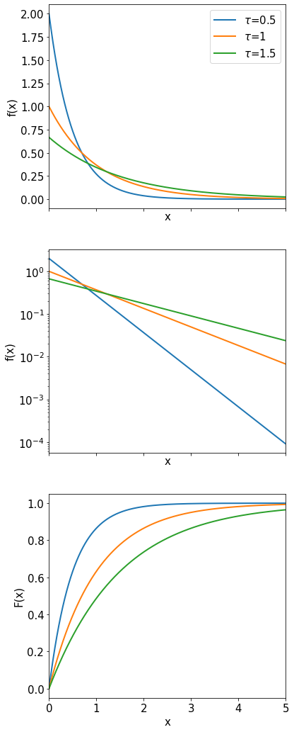
Exponential Distribution#
The exponential distribution is defined for a continuous variable \(t\) (\(0 \le t \le \infty\)) by:
The probability density is characterized by one single parameter \(\tau\).
The expectation value is \(\langle t \rangle=\frac{1}{\tau}\int_0^{\infty}te^{-t/\tau}dt=\tau.\)
The variance is \(\mbox{Var}(t)=\tau^2\).
An example for the application of the exponential distribution is the description of the proper-decay-time decay \((t)\) of an unstable particles. The parameter \(\tau\) corresponds in this case to the mean lifetime of the particle.
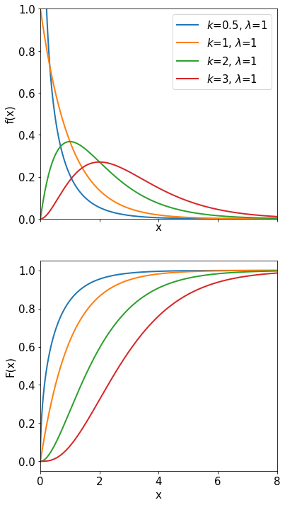
Gamma Distribution#
The gamma distribution is given by:
The expectation value is \(<x> = k / \lambda\).
The variance is \(\sigma ^{2} = k / \lambda^{2}\).
Special cases:
for \(\lambda = 1/2\) and \(k=n/2\) the gamma distribution has the form of a \(\chi^2\) distribution with n degrees of freedom.
The Gamma distribution describes the distribution of the time \(t=x\) between the first and the \(k^{th}\) event in a Poisson process with mean \(\lambda\). The parameter \(k\) influences the shape of the distribution, whereas \(\lambda\) is just a scale parameter.
Student’s \(t\)-distribution#
The Student’s \(t\) distribution is used when the standard deviation \(\sigma\) of the parent distribution is unknown and instead we use \(s\) evaluated from the sample. Suppose that \(x\) is a random variable distributed normally (mean \(\mu\), variance \(\sigma^{2}\)), and a measurement of \(x\) yields the sample mean \(\bar{x}\) and the sample variance \(s^{2}\). Then the variable \(t\) is defined as
We have repaced the unknown standard deviation of the parent distribution with estimated one.
The Student’s \(t\) distribution can be obtained from the ratio of two independent random variables: z at the numerator following a Normal distribution N(0,1) and v at the denominator following a \(\chi^2(n)\) with n degrees of freedom (sample size). The ratio
\(t = \frac{z}{\sqrt{V/n}} \)
follows a Student’s \(t\) distribution with n degrees of freedom (sample size).
To see this take n independent identically distributed samples from a Normal distribution \(N(\mu,\sigma^2)\). The sample mean \(\bar{x}\) follows a normal distribution \(N(\mu, \sigma^2/n)\), which can be standardized to N(0,1) by taking \(z = \frac{\bar{x} - \mu}{\sigma/\sqrt{n}}\).
The scaled sample variance \(V = \frac{(n-1)s^2}{\sigma^2}\) is distributed as a \(\chi^2_{n-1}\) (from the definition of Variance and from the fact that the \(\chi^2\) distribution is the distribution of the sum of the square of normally distributed random variables).
Now substitute them in \(t = \frac{Z}{\sqrt{V/\nu}}\):
\( t = \frac{\frac{\bar{x}-\mu}{\sigma / \sqrt{n}}}{\sqrt{\left(\frac{(n-1) s^2}{\sigma^2}\right) /(n-1)}} \)
Simplify the denominator to: \( \sqrt{\left(\frac{(n-1) s^2}{\sigma^2}\right) /(n-1)} = \frac{s}{\sigma}\)
and you get: \( t = \frac{\frac{\bar{x}-\mu}{\sigma/\sqrt{n}}}{s/\sigma} = \frac{\bar{x}-\mu}{s/\sqrt{n}} \)
The typical application of the Student’s t is in hypotesis testing to test the compatibility of the mean of a distribution with unknown standard deviation against a reference value \(\mu\).
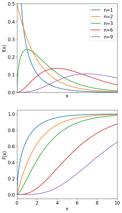
The p.d.f. of the Student’s t \(f_n(t)\) with \(n\) degrees of freedom is:
In the plot below note the larger tails compared with a gaussian. Intuitively one expects them because the true mean \(\sigma\) is replaced with the sample mean \(s\).
\(F\)-distribution#
Consider two random variables, \(\chi_1^2\) and \(\chi_2^2\), distributed as \(\chi^2\) with \(\nu_1\) and \(\nu_2\) degrees of freedom, respectively. We define a new random variable \(F\) as:
The random variable \(F\) follows the distribution:
This distribution is known by many names: Fisher-Snedecor distribution,
Fisher distribution, Snedecor distribution, variance ratio distribution,
and \(F\)-distribution. By convention, one usually puts the larger value
on top so that \(F \ge 1\).
The \(F\) distribution is used to test the statistical compatibility
between the variances of two different samples, which are obtained form
the same underlying distribution (more in Hypothesis testing).

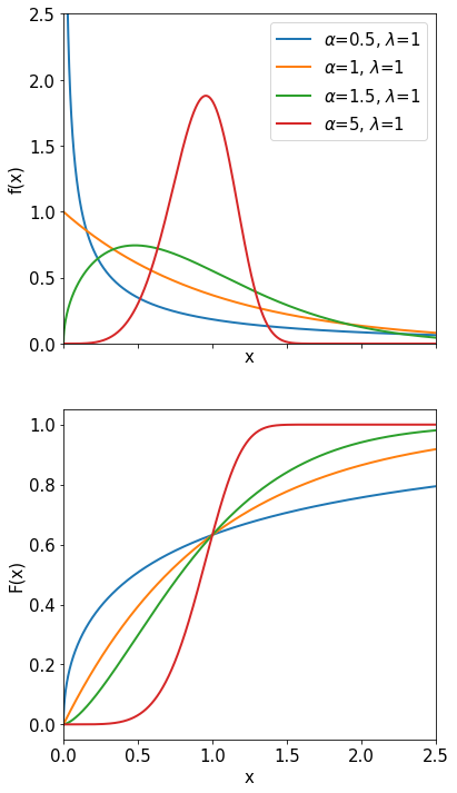
Weibull Distribution#
The Weibull distribution was originally invented to describe the rate of failures of light bulbs:
with \(x\ge 0\) and \(\alpha, \lambda > 0\). The parameter \(\alpha\) is just a scale factor and \(\lambda\) describes the width of the maximum. The exponential distribution is a special case \((\alpha = 1)\), when the probability of failure at time t is independent of t. The Weibull distribution is very useful to describe the reliability and to predict failure rates. The expectation value of the Weibull distribution is \(\Gamma(\frac{1}{\alpha}+1) \frac{1}{\lambda}\) and the variance is \(\frac{1}{\lambda^2} \left( \Gamma\left(\frac{2}{\alpha} +1\right) - \Gamma^2\left(\frac{1}{\alpha} +1\right) \right)\).
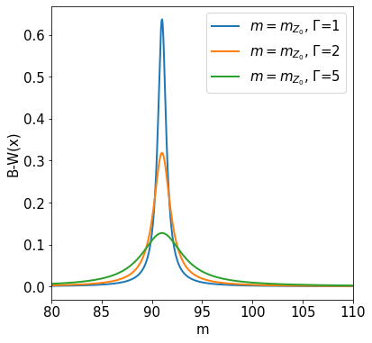
Cauchy (Breit-Wigner) Distribution#
The Cauchy probability density function is:
For large values of \(x\) it decreases only slowly. Neither the mean nor the variance are defined, because the corresponding integrals are divergent. The particular Cauchy distribution of the form
is also called Breit-Wigner function (see below), and is used in particle physics to describe cross sections near a resonance with mass \(M\) and width \(\Gamma\). The Breit-Wigner comes as the Fourier transformation of the wave function of an unstable particle:
which squared gives:
Landau Distribution#
The Landau distribution (see Fig. 4) is used to describe the distribution of the energy loss \(x\) (dimensionless quantity proportional to \(dE\)) of a charged particle (by ionisation) passing through a thin layer of matter:
The long tail towards large energies models the large energy loss
fluctuations in thin layers. The mean and the variance of the
distribution are not defined.
Often it can be found approximated as:
Fig. 4 Straggling functions in silicon for 500 MeV pions, normalized to unity at the most probable value \(\delta p/x\). The width \(w\) is the full width at half maximum. [Gro22a]#
Crystal Ball#
The Crystal Ball is typically used to describe the invariant mass distribution of a resonance in which the decay products are affected by energy losses. An example could be a \(Z\to e^+ e^-\) where the electrons in the final state lose energy by brehmstralung. The distribution is characterized by a Gaussian core with a power law tail
where:
A trivial extension is given by the “Double Crystal Ball” where a second exponential tail is added on the high side.
where:
In case you are wondering, the name comes from the collaboration that first used this function to describe a signal distribution. [@crystalBall].
The Central Limit Theorem#
The “Central Limit Theorem” (CLT) is probably the most important theorem
in statistics and it is the reason why the Gaussian distribution is so
important.
Take \(n\) independent variables \(x_i\), distributed according to p.d.f.’s
\(f_i\) having mean \(\mu_i\) and variance \(\sigma_i^2\), then the p.d.f. of
the sum of the \(x_i\), \(S=\sum x_i\), has mean \(\sum \mu_i\) and variance
\(\sum\sigma_i^2\) and it approaches the normal p.d.f.
\(N(S; \sum \mu_i, \sum \sigma_i^2)\) as \(n\to \infty\).
The CLT holds under pretty general conditions:
both mean and variance have to exist for each of the random variables in the sum
Lindeberg criteria:
\[\begin{split} \begin{aligned} y_k &=& x_k,\quad {\rm if}\, |x_k-\mu_k|\le \epsilon_k\sigma_k \\ y_k &=& 0,\quad {\rm if}\, |x_k-\mu_k|> \epsilon_k\sigma_k. \end{aligned} \end{split}\]Here, \(\epsilon_{k}\) is an arbitrary number. If the variance \((y_{1}+y_{2}+\cdots y_{n})/ \sigma_{y}^{2} \to 1\) for \(n \to \infty\), then this condition is fulfilled for the CLT. In plain English: The Lindeberg criteria ensures that fluctuations of a single variable does not dominate its sum.
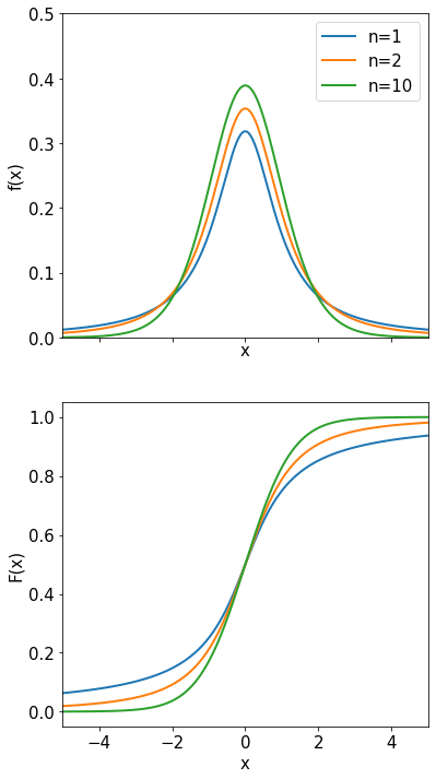
An example of convergence for the CLT is given below where a uniform distribution is used for 4 iterations.
When performing measurements the value obtained is usually affected by a large number of (hopefully) small uncertainties. If this number of small contributions is large the C.L.T. tells us that their total sum is Gaussian distributed. This is often the case and is the reason resolution functions are usually Gaussian. But if there are only a few contributions, or if a few of the contributions are much larger than the rest, the C.L.T. is not applicable, and the sum is not necessarily Gaussian.
Example:
The inverse transverse momentum \(q/p_T\), with q the charge of the particle, can be deduced from the measured sagitta. \(Q/p_T\) has Gaussian errors, not \(p_T\) !
References#
Pretty much every book about statistics/probability will cover the material of this chapter. Here are a few examples: