Monte Carlo methods

Monte Carlo methods#

In this chapter we will discuss an introduction to the so-called Monte Carlo (MC) simulations, which use random numbers and a sequential description of the operations as basic concepts. Because this method uses principles from probability calculations and statistics, it is also known as the method of statistical trials. In the next sections, after a digression on random number generators, we will describe two of the most common applications of Monte Carlo methods: integration and simulation.

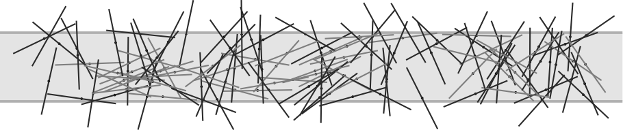
_images/needledisplay2.png — Fig. 7 Randomly distributed needles on a strip which has the width of the length of one needle. 81 out of 128 needles cross the border of the strip in this picture. Wikipedia#

Probably the oldest mentioning of a Monte Carlo method, which illustrates all its basic elements, is known as the needle experiment by Buffon. The duke baffled his colleagues in 1777 with a simple method to get the number $\pi$ by simply counting the number of needles thrown onto a strip with the same width as the length of the needles $(l)$. He found out that the ratio between the number of needles $(k)$ crossing the border of the strip (the slightly darker ones in Fig. 7) and the total number of thrown needles $(n)$ is exactly $2 / \pi$ (i.e. $k / n = 2 / \pi = p$). This value is calculated analytically using the position dependent probability density to cross the border of the strip, which is an $arccos$ function, mirrored in the middle of the strip (see Fig. 8. The picture on the right hand side in Fig. 8 shows the convergence to the exact value of $\pi$ with increasing number of thrown needles. The dashed line in this figure is the expected error for the value of $\pi$, which is calculated using the binomial distribution for $k$ by including the error propagation to be $\frac{2n}{k^{2}} \sqrt{np(1-p)} = 2.37 / \sqrt{n}$.

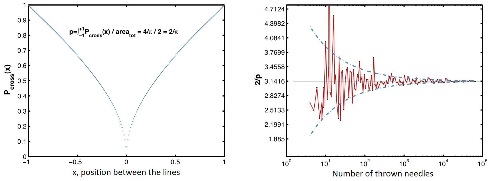
_images/needlemcEnglishRotatedPNG.png — Fig. 8 Probabilities for needles to cross the border of the strip depending on their position between the two borders (left), and the result of a MC simulation with its error (dashed line).#

Another example for the determination of $\pi$ is to inscribe a circle in a square and drop objects randomly on it (e.g. drops of rain, see Fig. 9. From the ratio of the number of drops ending in the circle to the total number of drops in the square one finds that $\pi = 4 * in / all$. With $10^6$ drops we found a value of 3.13954.

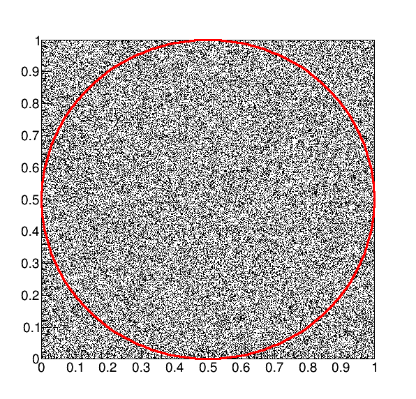
_images/piMC.png — Fig. 9 The circle inscribed in a square used to calculate $\pi$.#

As of today, the MC methods are preferably used in numerical mathematics if the formulation of the stochastic model is simpler than the formulation of the analytic model for the numerical solution of the problem. Monte Carlo methods are used in many different areas of research. To name just a few of them:

Numerical problems, such as the calculation of integrals or the solution of ordinary or partial differential equations.
Quality control of products, for example the determination of the lifetime of light bulbs.
Problems from operations research, such as transport problems.
Decision management using simulations or risk analysis in investment banking.

Monte Carlo methods can generally be spilt into three major steps:

A stochastic model has to be found for the original mathematical model, which describes the problem accurately enough.
A sequence of random numbers has to be generated, which are then used to simulate a realistic situation, and hence have the same underlying distribution.
Estimates for the original problem have to be found using the results coming from the random numbers.

Monte Carlo was eponymous for this process: the problems connected to gambling were motivating enough to start thinking about randomness of events.

(Pseudo)Random Numbers Generators#

True random generators are based on physical processes. Examples can be the noise level across a resistor, the time between the arrival of two cosmic rays or the number of radioactive decays in a fixed time interval. A method from the early applications of Monte Carlo technique in high energy physics, used the stopping azimuthal position of a cylinder which had been put in rotation by a motor (activated by an operator) and turned off by a cosmic ray recorded by a detector.

The main issues with these kind of random number generators is that they are very slow. The solution adopted is to generate random numbers running an algorithm on a computer. By construction the obtained random sequence is not random (that’s why they are called pseudo-random). We’ll see in the following that the two most important parameters of any generator are the period length (how many numbers it can generate before it starts to repeat itself) and the correlation between the generated numbers.

A simple and classic generator is the general linear congruential generator:

\[ n_{i+1}=(a\cdot n_{i}+c)\,\,\,\mathrm{mod}\,\,\,m\hspace{8mm} u_{i}=n_{i}/m \]

it generates uniformly distributed numbers in the interval (0…1]. The boundary value 0 is usually not included to avoid the divide-by-zero danger in case the number is carelessly used in further calculations. We will call such a uniform probability density $U(0,1)$:

\[\begin{split} \begin{aligned} U(0,1) = \begin{cases} 1 \qquad &\text{if} \hspace{2mm}0<u\le1, \\ 0 &\text{else} \end{cases} \end{aligned} \end{split}\]

The algorithm uses three integer constants: the multiplicand $a$, the summand $c$ and the module $m$. Generators with the summand $c = 0$ are called multiplicative linear congruential generators. The initial value $n_{1}$ is also called seed: the choice of the initial value allows to steer the generation process. The distribution and the correlation among the first 10’000 values using the values $m = 2^{31}$, $a=65539$ and $c=0$ is shown in Fig. 10 . It was first used in the sixties by IBM and became famous under the name of RANDU, but it had bad performance.

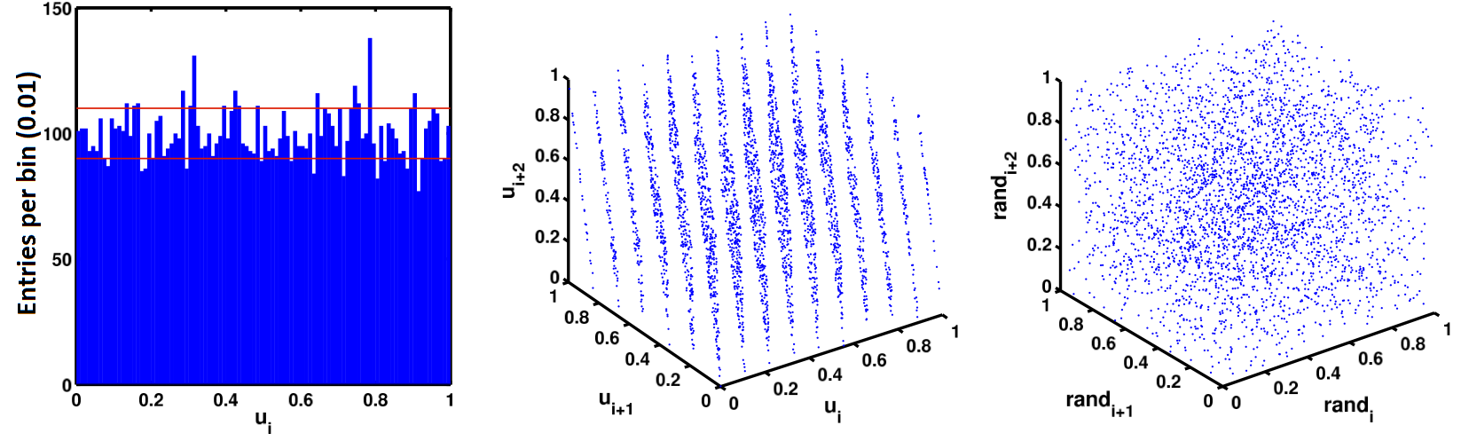
_images/mulincongPNG.png — Fig. 10 Histogram (100 bins) of the first 10’000 values generated with *RANDU* and correlations among three sequential values (not binned). 10’000 values, generated with the Mersenne Twister-function, have been plotted for comparison in the same way on the right hand side graph. Wikipedia#

$k$-tuple of random numbers lies in the $k$-dimensional space on $(k-1)$-dimensional hyperplanes. The maximal distance between these hyperplanes is an important test for linear generators (spectral test). The graph on the right hand side in Fig. 10 compares RANDU (graph in the middle) to a far more uniform distribution from the Mersenne Twister generator.

Nowadays algorithms exist with a period length of $2^{19937}$ and which are (for most practical purposes) uncorrelated. The random generators which are implemented in many computer programs are usually sufficient for daily use. Nevertheless, in some special cases such as cryptography, better generators are needed.

Two tricks used to get random numbers with minimal correlation and extraordinary long period length are:

Combination: Two random numbers are generated with a generator each, and a new one is generated using the operations $+$, $-$ or exclusive-OR at bit level.
Rearrangement: The memory is filled with some random numbers, and the result of another generator is used to determine the address in the memory for the next random number.

Tests of Random Generators#

Among the most important ones are:

Test for uniform distribution. The interval [0,1] is divided into $k$ equal sub-intervals of length $1/k$. $N$ random numbers $u_{i}$ are generated and it is counted how many of these numbers come to lie in each of the sub-intervals. If we call the number of cases in each sub-interval $N_{i}$, $i$ = 1 … $k$, then the sum

\[ \chi^{2}=\sum_{i=1}^{k}\frac{(N_{i}-N/k)^{2}}{N/k} \]

should (for $N / k \geq 10)$ approximately follow a $\chi^{2}$-distribution with ($k$-1) degrees of freedom. This means that on average the ratio $\chi^{2} / (k-1)$ should be 1. Similar expressions can be constructed for non-uniform distributions.
Test for correlation. If $n$ successive random numbers are plotted as coordinates in an $n$-dimensional space, then these points lie on hyperplanes, as shown above. A good generator has many hyperplanes which are uniformly distributed.

Gap test. Choose two numbers $\alpha, \beta$ with $0 \leq \alpha < \beta \leq 1$. Generate $r+1$ random numbers, which are uniformly distributed in the interval [0,1]. The probability that the first $r$ numbers are not included in the interval $[\alpha, \beta]$ and the last, $r+1^{st}$ number is included in the interval should be $P_{r}=p(1-p)^{r}\,\,\,\rm{with}\,\,\, p=\beta -\alpha$.
Random walk test Choose a number $0 < \alpha <1$. Build a large set of random numbers and note the number of cases $r$ in which a random number is smaller than $\alpha$. We expect this to be a binomial distribution for $r$ with $p = \alpha$. This test is very sensible for large values of $r$. The test should also be made for the amount of random numbers which are larger than $(1-\alpha)$.

Arbitrarily distributed Random Numbers#

Up to now we considered random numbers generated on a constant distribution. More generally we will need random numbers distributed according to some probability density $f(x)$. For example, we might need random numbers following a Gaussian distribution. In this section we will describe the most important methods to generated arbitrarily distributed random numbers.

Inverse of the Cumulative Distribution#

A standard procedure to produce random numbers generated according to the distribution $f(x)$ starts with random numbers $u_{i} \in U(0,1)$ and transforms them using the inverse function of the cumulative distribution $F(x)$:

\[ f(x)\, dx = U(0,1)\,du\hspace{15mm}\int_{-\infty}^{x}f(t)\,dt = F(x) = u \hspace{15mm} x = F^{-1}(u) \]

$F^{-1}$ is the inverse function of the cumulative distribution function $F(x)$. The method is illustrated in Fig. 11. For a sequence of uniform random numbers $u_{i}$, the random numbers $x_{i} = F^{-1}(u_{i})$ are distributed according to the probability density $f(x)$. In practice one matches the first x-% quantile of the first distribution to the x-% quantile of the target distribution $f(x)$.

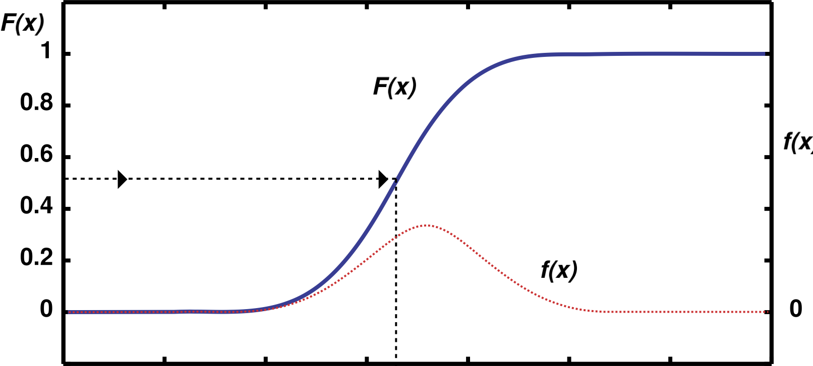
_images/invFtrans.png — Fig. 11 Generation of random numbers on a continuous distribution $f(x)$ using the inverse of the cumulative distribution function $F(x)$.#

This method can only be applied if the integral of the probability density can be expressed as an analytic function $F(x)$ and this $F(x)$ is invertible.

Example:

Random numbers generated on an exponential distribution. The p.d.f. for the exponential distribution is given by the $f(x;\lambda) = \lambda e^{-\lambda x}$ for $x\geq 0$, and it is zero for $x<0$. The cumulative distribution is:

\[ u= F(x;\lambda) = \int _{0}^{x}\lambda e^{-\lambda t} dt=1-e^{-\lambda x} \]

Inverting the cumulative we get the sequence of exponentially distributed random numbers $x_{i} = - \ln (1 - u_{i} )/ \lambda$. Or, because $u_{i}$ and $1-u_{i}$ are equally distributed in the interval $(0...1)$ we can write $x_{i} = - \ln(u_{i}) / \lambda$.

If we have an application with very large random numbers (for example very long lifetimes $t \gg \tau = 1 / \lambda)$, then the above method might not be precise enough. Very large values of $x$ are generated by very small values of $u$. Because floating point numbers are represented with finite accuracy in a computer, large values of $x$ will appear as discrete.

Acceptance-Rejection Method#

The acceptance-rejection method (also known as “hit-or-miss”), even though not very efficient, can be used to generate random numbers according to a given probability density $f(x)$ when the cumulative distribution function $F(x)$ cannot be inverted.
Under the assumption that the variable $x$ is restricted to some interval $a < x < b$, we can determine an upper limit $c$ with $c \geq \max(f(x))$; where $\max(f(x))$ is the maximum of $f(x)$ in the interval $[a,b]$. This is then fed into the following algorithm:

Choose $x_{i}$ uniformly from the interval [a,b]: $x_{i} = a + u_{i} \cdot (b-a)$.
Choose another random number $u_{j} \in U(0,1)$.
If $f(x_{i}) < u_{j} \cdot c$, then go back to step 1, otherwise accept $x_{i}$ as random number.

The efficiency of this method is given by the ratio between the integral of $f(x)$ over [a,b] and the total area $c \cdot (b-a)$ of the space of all generated pairs $(u_{i}, u_{j})$. The efficiency can be increased if we can find a function $s(x)$ which has the approximate shape of $f(x)$, which has an invertible cdf and for all $x$ in [a,b] and $s(x) > f(x)$. By means of $$\int_{-\infty}^{x}s(t)dt=S(x)\hspace{20mm}x_{i}=S^{-1}(u_{i})$$ we can apply the following algorithm:

Choose a random number $u_{i}$ and calculate $x_{i} = S^{-1}(u_{i})$.
Choose another random number $u_{j} \in U(0,1)$.
If $f(x_{i}) \leq u_{j} \cdot s(x_{i})$, then go back to step 1, otherwise accept $x_{i}$ as random number.

The random number $x_{i}$ corresponds to the $s(x)$-distribution. The probability that it is accepted in step 3 is so increased because we better target the generation of the sampling points.
Choosing an envelope for the generation of the sampling points is particularly useful in case of steeply falling or very “irregular” distributions.

Specially distributed Random Numbers#

A random angle $\phi$, distributed in $[0, 2 \pi]$, is obtained by $\phi_{i} = 2 \pi \cdot u_{i}$. The random unit vector is then simply:

\[ \cos \phi_{i} \choose \sin \phi_{i} \]

In three dimensions, an additional polar angle $\theta \in [- \pi / 2, \pi / 2]$ is needed (in addition to sin $\phi$ and cos $\phi$). According to the differential solid angle

\[ d\Omega = {\rm sin}\theta\, d\theta\, d\phi = |d\,{\rm cos}\theta|\, d\phi \]

we obtain $\theta_{j} = {\rm arcsin} (2 \cdot u_{j} -1)$ from the analytical transformation. For the 3 components of the random unit vector we get $e_{x} = \sin \phi \cdot \cos \theta$, $e_{y} = \cos \phi \cdot \cos \theta$ and $e_{z} = \sin \theta$.

This is one of the most commonly used distribution for random numbers. The simplest but only approximately correct generator for the random numbers $z_{i}$, which are distributed according to a Gaussian distribution ($1 / \sqrt{2 \pi} \cdot e^{-x^{2}/2}$) in the interval [-6,6], is based on the central limit theorem:

\[ z_{i}=\sum_{j=1}^{12}u_{j}-6 \]

Random numbers in ROOT and PYTHON#

ROOT (TRandom3) and PYTHON (import random) use the Mersenne Twister algorithm wiht a period of $2^{19927}-1 \sim 4.3 \cdot 4.3 10^{6001}$ equidistributed in up to 623 dimensions (for 32-bit machines). Both ROOT and PYTHON have predefined functions to generate numbers according to the most common pdf.

Monte Carlo Integration#

Monte Carlo techniques can be used to evaluate (definite) integrals:

\[ I = \int_a^b f(x) dx \]

with $f(x)$ is any function. The straightforward deterministic way to evaluate the integral is to divide the range $[a,b]$ in n intervals and compute $I$ as:

(5)#\[\frac{b-a}{n}\sum_{i=1}^n f(x_i)\]

where $x_i = a+(i-0.5)(b-a)$. This is what is typically called the method of the trapezoid. You can evaluate the funciton at the central value of the bin, or at the min and max and approximate the function with a linear interpolation, etc …

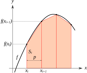
_images/trapezoid.png — Fig. 12 Definite integral computed with the trapezoid method Wikipedia#

The uncertainty on the integral goes as $n^{-2}$ in one dimension.

The most naive implementation of the Monte Carlo way of computing the integral differs in the choice of the points where we evaluate the sum: instead of regularly spaced points we randomly sample the axis:

\[ x_i = a+ r_i (b-a) \]

with $r_i$ random numbers uniformly distributed in $[0,1]$.

The first consequence of this approach is that the result is non deterministic: different sequences of random numbers will give different integral values.

The uncertainty on the estimate of the integral $I$ can be estimated as the variance of $f(x_{i})$ in the following way:

\[ V[I_{MC}]=\sigma_{I_{MC}}^{2}=V\Big[\frac{b-a}{n}\sum_{i=1}^{n}f(x_{i})\Big]= \Big(\frac{b-a}{n}\Big)^{2}V\Big[\sum_{i=1}^{n}f(x_{i})\Big]=\frac{(b-a)^{2}}{n}V[f(x_{i})] \]

This equation shows us that the accuracy of the computation decreases with $1/\sqrt{n}$.

To compute integrals in larger dimensions with the trapezoidal method you need to create an d-dimensional equidistand grid of points, evaluate the function at those points and sum over the d-dimensional trapezoid. The uncertainty of the trapezoidal method in d-dimensions goes as $n^{-2/d}$, while the uncertainty of the Monte Carlo approach is $1/\sqrt{n}$ in any dimension.

Methods to reduce the Variance#

The Monte Carlo integration shown above is just the most naive implementation of this technique. There are several ways to improve the numerical result (reducing the variance)

Simply dividing the range of integration in two regions and generating half of the Monte Carlo points in each of the regions reduces the variance. The reason is that in this way we allow a more uniform sampling of the distribution.

Given that we know how the integrand $f(x)$ behaves, we can sample the distribution with higher density of random points where the function is varying more rapidly. It’s like in the stratification but this time the intervals are chosen in a more cleverer way.

Because the variance of the Monte Carlo result is proportional to the variance of the integrand, it makes sense to transform the integral to get a new integral with a smaller variance than the original one. By introducing a function $g(x)$ we can write:

\[ \begin{aligned} \int_{a}^{b} f(x)dx=\int_{a}^{b} \Big[\frac{f(x)}{g(x)}\Big]g(x)dx = \int_{A}^{B} \Big[\frac{f(x)}{g(x)}\Big]dv(x) \quad \text{with }v(x)=\int g(x)dx \end{aligned} \]

The variance of the new result is now proportional to the one of $f(x)/g(x)$ instead of being proportional to $f(x)$ alone. If $g(x)$ has been chosen carefully, the method of importance sampling allows us to reduce the variance of the Monte Carlo integration considerably. But the function $g(x)$ has to be integrable and invertible, and it has to describe the original function $f(x)$ appropriately enough.

This is similar to importance sampling except that instead of dividing by g(x) subtract it:

\[ I = \int f(x) dx = \int [f(x) - g(x)] dx + \int g(x) dx \]

Here $\int g(x) dx$ must be known and $g$ is chosen such that $f-g$ has a smaller variance than $f$. This method does not risk the instability of importance sampling, nor is it necessary to invert the integral of $g(x)$.

Up to now the Monte Carlo points were all independent. But looking at the variance of two general functions:

\[ V[f_1(x)+f_2(x)] = V[f_1(x)] + V[f_2(x)] + 2cov[f_1(x),f_2(x)] \]

and writing the integral as $I = \int_a^b f = \int_a^b(f_1 + f_2) dx$ we observe that we can reduce the covariance of $I$ by introducing a large negative correlation.

Example:

Suppose that we know that $f(x)$ is a monotonically increasing function of $x$. Then let $f_1 = 1/2 f(x)$ and $f_2 = 1/2 f(b-(x-a))$. Clearly the integral of $(f_1 +f_2)$ is just the integral of $f$. However, since $f$ is monotonically increasing, $f_1$ and $f_2$ are negatively correlated; when $f_1$ is small, $f_2$ is large and vice versa. If this negative correlation is large enough, $V [f_1 + f_2] < V [f]$.

Monte Carlo Simulations#

We will briefly describe in this section the typical applications of Monte Carlo techniques in high energy physics: simulation of a physics process, simulation of a detector, study of reconstruction programs, physics reach of an experiment, “toy” experiments.

Simulation of a physics process#

In particle physics, “generators” are programs used to simulate the production (and decays) of particles. The generators allow to compute the full kinematics of the process and to get the distributions of the observables, which are typically impossible to derive with analytical methods. The description of a proton proton collision for example requires the understanding of several components: the hard scatter (matrix elements + pdf), initial/final state radiation, parton showering and hadronization and decays of the generated final states. This kind of process can be treated only with Monte Carlo simulations. An introduction to Monte Carlo generators in high energy physics can be found in [@MCgen].

Simulation of a detector#

Once the particles are generated we will need to understand how they will be “seen” by a detector. This requires basically two steps, which in jargon are called “simulation” and “digitization”. In the first the particles are propagated through the detector simulating their interactions with all sensitive and passive materials. For instance a high energy photon hitting a calorimeter will create an electromagnetic shower, while a charged particle will deposit a fraction of its energy in a silicon layer. These phenomena are simulated with standard programs like GEANT or FLUKA, MARS etc… which contain software libraries describing the details of the interactions. The digitization step simulates how the energy deposited in the different sensitive material is transformed into electric/optical signals. In this case the signals are a mixture of deterministic effects (e.g. amplification/shaping) overlapped with random effects (e.g. noise or finite accuracy of calibrations) described with Monte Carlo methods.

Study of reconstruction programs#

The electronic signals can then be analysed to “reconstruct” physics objects. Those can be e.g. the tracks of charged particles in a tracker, or the electromagnetic showers in a calorimeter. Even in this case, Monte Carlo simulations are essential tools to develop the reconstruction software. In this case, starting from Monte Carlo samples of particles, and so knowing exactly their type and their kinematics, we can develop the reconstruction packages to be able to reconstruct them with high efficiency and accuracy.

Physics reach of an experiment#

Simulations are not important only to decipher the results of an experiment once the data are collected. They are the first necessary step in the design of an experiment. The conception of a detector starts with simulations where different solutions can be tested without doing the actual prototypes, which would be unacceptably expensive and time consuming.

Toy modelling#

“A good physicist knows how to build toy models.” This quotation from an anonymous physicist summarize the importance of toy modeling in physics. Toys can be used to get a first understanding of a process picking only its essential characteristics (here is where the physicist has to be good) and avoiding all complications of real experimental life. As it will be seen in hypothesis testing, toys are also an ubiquitous tool used in statistics for hypothesis testing.

References#

Most of the material of this section is taken from:

L. Lyons, [Lou86], “Statistics for Nuclear and Particle Physicist”: Ch. 6
T. Sjostrand, [Sjo12], “Introduction to Monte Carlo techniques in High Energy Physics”