Hypotheses Testing

In the previous chapters we used experimental data to estimate parameters. Here we will use data to test hypotheses. A typical example is to test whether the data are compatible with the theoretical prediction or to choose among different hypothesis which one best represents the data.

Hypotheses and tests statistics

Let’s begin by defining some terminology that we will need in the following. The goal of a statistical test is to make a statement about how well the observed data stand in agreement (accept) or not (reject) with a given predicted distribution, i.e. a hypothesis. The typical naming for the hypothesis under test is the null hypothesis or \(H_{0}\). The alternative hypothesis, if there is one, is usually called \(H_{1}\). If there are several alternative hypotheses they are labeled \(H_{1}, H_{2}, \ldots\)

Example:

When testing data for the presence of a signal, we define the null hypothesis as the “background only” hypothesis and the alternative hypothesis as the “signal+background” hypothesis.

Example:

Fig. 20 shows the cross section \(\sigma(e^+e^-)\to W^+W^-(\gamma)\) measured by the L3 collaboration at different centre of mass energies. In this case the test statistic is the cross-section as a function of energy. The measured values are then compared with different theoretical models (different hypothesis). We haven’t explained yet how to quantitatively accept or reject an hypothesis, but already at a naive level we can see that data clearly prefer one of the models.

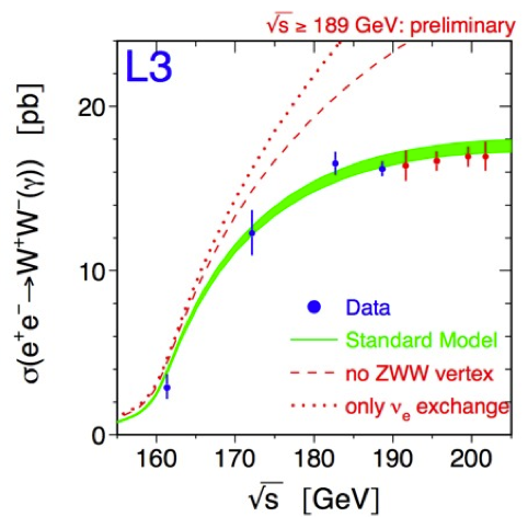
Fig. 20 Analysis of the cross section of \(e^+e^-\to W^+W^-(\gamma)\) as a function of the centre of mass energy (L3 detector at LEP).

The hypothesis can be simple if the p.d.f. of the random variable under test is completely specified (e.g. test for the existence of a new particle with all specified properties) or composite if at least one of the parameters is not specified (e.g. test for the existence of a new particle of unknown mass).

To quantify the agreement between the observed data \(\vec{x}\) and a given hypothesis, we construct a function \(t(\vec{x})\): the test statistics.

If we build it in a clever way, the test statistic will be distributed differently depending on the hypothesis under test: \(g(t(\vec{x})|H_0) \neq g(t(\vec{x})|H_1)\). This pedantic notation is used here to stress that the test statistic is a function of the data and that it is the distribution of the test statistic values that is different under the different hypotheses (the lighter notation \(g(t|H_i)\) will be used from now on).

Example:

In order to better understand the terminology we can use a specific example based on particle identification. The average specific ionization \(dE/dx\) of two charged particle with the same momentum passing through matter will be different depending on their masses (see Fig. 21, \(\beta\gamma = p / m\)). Because of this dependence \(dE/dx\) can be used as a particle identification tool to distinguish particle types. For example the ionization of electrons with momenta in the range of few GeV tend to be larger than the one of pions of the same momentum range.

If we want to distinguish an electron from a pion with a given momentum we can use the specific ionization itself as test statistic \(t(\vec{x}) = dE/dx\). This is a typical case where the data itself is used as test statistic. The test statistics will then be distributed differently under the two following hypotheses (see Fig. 22):

• null hypothesis \(g(t|H_0) = P\left(\frac{dE}{dx}|e^{\pm}\right)\)

• alternative hypothesis \(g(t|H_1) = P\left(\frac{dE}{dx}|\pi^{\pm}\right)\)

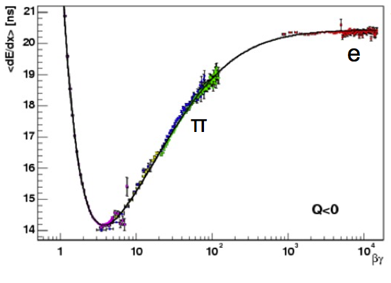
Fig. 21 The specific ionization for some particle types (pions in green, electrons in red; other particles species are shown with different colors: protons in purple, kaons in blue, muons in yellow)

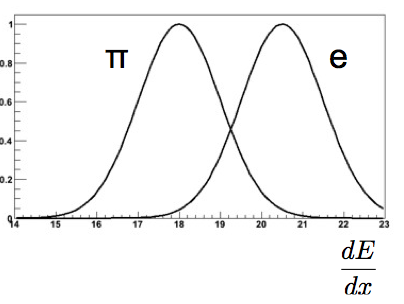
Fig. 22 The projections of Fig. 21 plot on the y-axis for electrons and pions, i.e. their measured specific ionization.

The test statistic can be any function of the data: it can be a multidimensional vector \(\vec{t}(\vec{x})\) or a single real number \(t(\vec{x})\). As seen in the example above, even the data themselves \(\{\vec{x}\}\) can be used as a test statistic. Collapsing all the information about the data into a single meaningful variable is particularly helpful in visualizing the test statistic and the separation between the two hypothesis.

There is no general rule about the choice of the test statistic. The specific choice will depend on the particular case at hand. Different test statistic will give in general different results and it is up to the physicist to decide which is the most appropriate for the specific problem.

The p.d.f. describing the test statistic corresponding to a certain hypothesis \(g(\vec{t}|H)\) is usually built from a data set that has precisely the characteristic associated to that hypothesis. In the particle identification example discussed before, the data used to build the p.d.f. for the two hypotheses were pure sample of electrons and pure samples of pions.

In a test beam, a beam of particles is prepared in a well defined condition (particle type, energy, etc…) and it is typically used to test a device under development. This configuration inverts the typical experimental conditions where a device with known properties is used to characterize particles in a beam or from collisions.

For example you can get a pure sample of electrons selecting tracks from photon conversions \(\gamma \to e^+ e^-\) and a pure sample of pions from the self-tagging decays of charmed mesons \(D^{*+}\to \pi^+ D^0; D^0\to K^- \pi^+ (D^{*-}\to \pi^- D^0; D^0\to K^+ \pi^-)\) (self-tagging means that by knowing the charge of the \(\pi\) in the first decay you can unambiguously assign the pion/kaon hypothesis to the positive/negative charge of the second decay). In other cases the p.d.f. are built from dedicated measurement (e.g. a test beam) or from Monte Carlo simulations.

Important remark:

In physics/science we cannot meaningfully accept an hypothesis: we can only reject them. E.g. we will never be able to say that the 125 resonance discovered at the LHC in 2012 is the SM Higgs boson. The reason is that its properties could deviate from the SM predictions by an amount not yet experimentally accessible.

The logic used to check the hypotheses is “reversed”, i.e. you always check that an hypothesis is not consistent with data. e.g: If the data are not in agreement with background predictions, then there is something else: a signal !

Significance, power, consistency and bias

Now that we have the concept of test statistics and its distribution under a given hypothesis, we can quantitatively decide if we accept or reject the statement that data are distributed according to the given hypothesis.

To do this we partition the space of the test statistics values into a critical region and its complementary the acceptance region (see Fig. 23). The value of the test statistics chosen to define the two regions is called decision boundary: “\(t_{cut}\)”. If the value of the test statistic computed on the data under test falls in the rejection region, then the null hypothesis is discarded, otherwise it is accepted (or more precisely not rejected).

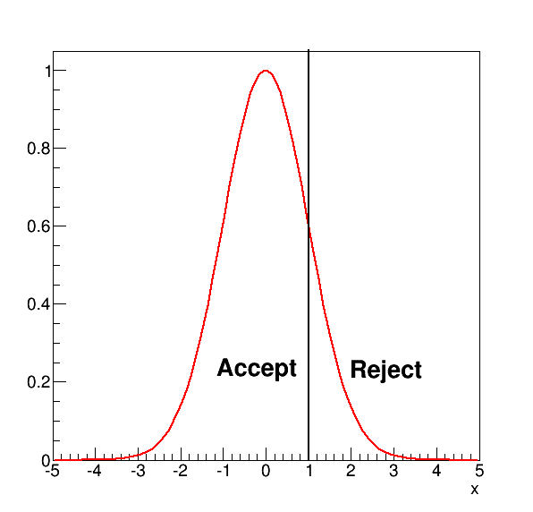
Fig. 23 A test statistic in red, where we defined an acceptance \(x\le 1\) and rejection region \(x>1\).

To decide the rejection region we will introduce two quantities: significance and power of the test.

The first one is the significance of the test (see Fig. 24). It is defined as the integral of the null hypothesis p.d.f. above the decision boundary:

\[\alpha = \int_{t_{cut}}^\infty g(t|H_0)dt \]

Fig. 24 Illustration of the acceptance and rejection region for the hypothesis \(H_{0}\).

The probability \(\alpha\) can be read as the probability to reject \(H_0\) even if \(H_0\) is in reality correct. This is called an error of the first kind.

If we have an alternative hypothesis \(H_1\), an error of the second kind occurs when \(H_0\) is accepted but the correct hypothesis is in reality the alternative one \(H_1\). The integral of the alternative hypothesis p.d.f. below \(t_{cut}\) is called the power of the test to discriminate against the alternative hypothesis \(H_1\) (see Fig. Fig. 25):

\[\beta = \int_{-\infty}^{t_{cut}} g(t|H_1)dt\]

Fig. 25 Illustration of the acceptance and rejection region the alternative \(H_{1}\).

A good test has both \(\alpha\) and \(\beta\) small, which is equivalent to say high significance and high power. This means that \(H_{0}\) and \(H_{1}\) are “well separated”.

Example:

Search for new physics: you analyse a mass spectrum looking for a bump. The null hypothesis is that data contains only background (see Fig. Fig. 26).

Type I error: there’s really no resonance, but you reject H0 and you announce a non existing discovery

Type II: there is a real resonance, you accept H0 and you miss the Nobel prize

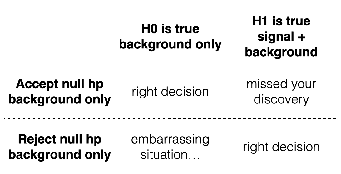
Fig. 26 Example of errors of the first and second kind in search for new physics.

While errors of the first type can be controlled by choosing \(\alpha\) as small as you want, errors of the second type depend on the separation between the two hypothesis and are not as easily controllable.

The typical criticism coming with this choice is on how we can be sure that we control the test statistics to such extreme tails. The typical answer is that such small values allow to a certain extent to also cover for possible mis-estimations of systematic uncertainties. It’s all hand-waving. The choice of the threshold to claim a discovery remains subjective.

In HEP searches we typically speak of “evidence” when \(\alpha \leq 3\cdot 10^{-3}\), and of “discovery” when \(\alpha \leq 3\cdot 10^{-7}\) (corresponding to the probability outside 3 \(\sigma\) and 5 \(\sigma\) respectively in a single sided tail Gaussian); these numbers are purely conventional and they don’t have any scientific ground. They are defined this way to set a high threshold for such important claims about the observation of new phenomena.

Example in Quality Control:

Consider a machine BM1 which is used for bonding wires of Si-detector modules. The produced detectors had a scrap rate of \(P_{0} = 0.2\). BM1 should be replaced with a newer bonding machine called BM2, if (and only if) the new machine can produce detector modules with a lower scrap rate \(P_{1}\). In a test run we produce \(n=30\) modules. To verify \(P_{1} < P_{0}\) statistically, we use the hypothesis test discussed above. Define the two hypotheses \(H_{0}\) and \(H_{1}\) as:

\[H_{0} : P_{1} \geq 0.2; \quad H_{1}: P_{1} < 0.2.\]

We choose \(\alpha = 0.05\) and our test statistic \(t\) is the number of malfunctioning detector modules. This quantity is distributed according to a binomial distribution, with the total number of produced modules \(n=30\) and a probability \(P\). The rejection region for \(H_{0}\) is constructed out of

\[ \sum_{i=0}^{n_c}{n \choose i}P_0^i(1-P_0)^{n-i}<\alpha.\]

Here, the critical value is denoted by \(n_{c}\), and it is the maximal number of malfunctioning modules produced by BM2 which still implies a rejection of \(H_{0}\) with CL \(1-\alpha\). By going through the calculation we find that for \(n_{c} =2\) the value of \(\alpha\) is still just below 0.05. This means that if we find two or less malfunctioning modules produced by BM2 we should replace BM1 by the new machine BM2.

Once the test statistics is defined there is a trade-off between \(\alpha\) and \(\beta\), the smaller you make \(\alpha\) the larger \(\beta\) will be; it’s up to the experimenter to decide what is acceptable and what is not.

Example:

Suppose we want to distinguish \(K-p\) elastic scattering events from inelastic scattering events where a \(\pi^0\) is produced:

\(H_0 : K^- p \to K^- p\)

\(H_1 : K^- p \to K^- p \pi^0\).

The detector used for this experiment is a spectrometer capable of measuring the momenta of all the charged particles (\(K^-\), \(p\)) but it is blind to neutral particles (photons from the \(\pi^0 \rightarrow \gamma\gamma\) decay). The considered test statistic is the “missing mass” \(M\) defined as the difference between the initial and final visible mass. The true value of the missing mass is \(M=0\) under the null hypothesis \(H_0\) (no \(\pi^0\) produced) and \(M_{\pi^0}=135~MeV/c^2\) under the alternative hypothesis \(H_1\) (a \(\pi^0\) is produced). The critical region can be defined as \(M>M_c\). The value of \(M_c\) depends on the significance and power we want to obtain (see Fig. 27): a high value of \(M_c\) will correspond to a high significance at the expenses of the power, while low values of \(M_c\) will result in a high power but low significance.

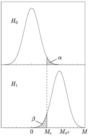
Fig. 27 Top: the p.d.f. for the test statistic \(M\) under the null hypothesis of elastic scattering \(H_0\) centred at \(M=0\); bottom the p.d.f. for the test statistic under the alternative hypothesis of inelastic scattering \(H_1\) centred at \(M=m_{\pi^0}\). \(M_c\) defines the critical region.

Some caution is necessary when using \(\alpha\). Suppose you have 20 researchers looking for a new phenomenon which “in reality” does not exist. Their \(H_0\) hypothesis is that what they see is only background. One of them could reject \(H_0\) with \(\alpha = 5\%\), while the other 19 will not. This is part of the game and therefore, before rushing for publication, that researcher should balance the claim with what the others don’t see. That’s the main reason why anytime there is a discovery claim, we always need to have the results to be corroborated by independent measurements. We will come back to this point when we will talk about the look-elsewhere effect.

Example:

Let’s use again the example of the electron/pion separation. As already shown before the specific ionization \(dE/dx\) of a charged particle can be used as a test statistic to distinguish particle types, for example electrons (\(e\)) from pions (\(\pi\))(see Fig. 21). The selection efficiency is defined as the probability for a particle to pass the selection cut:

\[\epsilon_e = \int_{-\infty}^{t_{cut}}g(t|e) dt = 1-\alpha \qquad \epsilon_\pi = \int_{-\infty}^{t_{cut}}g(t|\pi) dt = \beta\]

By moving the value of \(t_{cut}\) you can change the composition of your sample. The lower the value of \(t_{cut}\) the larger the electron efficiency but the higher the contamination from pions and vice-versa. In general, one can set a value of \(t_{cut}\), select a sample and work out what is the fraction of electrons \(N_{acc}\) present in the initial sample (before the requirement \(t<t_{cut}\)). The number of accepted particles in the sample is composed by:

\[N_{acc}=\epsilon_e N_e + \epsilon_\pi N_\pi = \epsilon_e N_e + \epsilon_\pi(N_{tot} - N_e)\]

which gives

\[N_{e}=\frac{N_{acc} - \epsilon_\pi N_{tot}}{\epsilon_e - \epsilon_\pi}\]

From this, one can immediately notice that the \(N_e\) can only be calculated if \(\epsilon_e \neq \epsilon_\pi\), i.e. \(N_e\) can only be extracted if there is any separation power at all. If there are systematic uncertainties in \(\epsilon_e\) or \(\epsilon_\pi\) these will translate into an uncertainty on \(N_e\). One should try to select the critical region \(t_{cut}\) such that the total error on \(N_e\) is negligible.

The other side of the problem is to estimate the purity \(p_e\) of the sample of candidates passing the requirement \(t<t_{cut}\):

\[\begin{split} \begin{aligned} p_e &=& \frac{\#electrons~with~t<t_{cut}}{\#particles~with~t<t_{cut}}\\ &=& \frac{\int_{-\infty}^{t_{cut}}a_e g(t|e) dt }{\int_{-\infty}^{t_{cut}}(a_e g(t|e) + (1-a_e)g(t|\pi) ) dt }\\ &=& \frac{a_e\epsilon_e N_{tot}}{N_{acc}} \end{aligned} \end{split}\]

Historically, in high energy physics a parallel nomenclature has been defined to express the same concepts we have encounter in this section:

• signal efficiency = 1-\(\alpha\) (a test is significant at a level 1-\(\alpha\) %)

  • \(\alpha\) = probability of a type I error

• background efficiency = \(\beta\) = probability of a type II error

  • 1-\(\beta\) = power of the test = background rejection

Is there a signal ?

A typical application of hypothesis testing in high energy physics is to test for the presence of a signal in data. The easiest case is represented by counting experiments. In this type of experiments the detector is used to count the number of events satisfying some selection criteria (slang: “cut-and-count”).

The signal doesn’t always appear as an excess of events. In case of test for neutrino oscillations the signal can appear as a deficit of events.

The number of expected events in case of background only hypothesis is compared with the measured number. The signal would typically appear as an excess over the expected background.

Example:

Let \(n\) be a number of events which is the sum of some signal and some background events \(n = n_s + n_b\). Each of the components can be treated as a Poisson variable \(\nu_s\) (signal) and \(\nu_b\) (background) and so the total \(\nu = \nu_s + \nu_b\) is also a Poisson variable. The probability to observe \(n\) events is:

\[f(n; \nu_s, \nu_b) = \frac{(\nu_s+\nu_b)^n}{n!}e^{-(\nu_s+\nu_b)}\]

Suppose you measure \(n_{obs}\) events. To quantify our degree of confidence in the discovery of a new phenomenon, i.e. \(\nu_s\ne 0\), we can compute how likely it is to find \(n_{obs}\) events or more from background alone.

\[P(n\ge n_{obs}) = \sum_{n=n_{obs}}^\infty f(n; \nu_s = 0, \nu_b) = 1 - \sum_{n=0}^{n_{obs}-1} f(n; \nu_s = 0, \nu_b) = 1- \sum_{n=0}^{n_{obs}-1} \frac{\nu_b^n}{n!}e^{-\nu_b}.\]

For example, if we expect \(\nu_b = 0.5\) background events and we observe \(n_{obs} = 5\), then the p-value is \(1.7 \cdot 10^{-4}\). This is not the probability of the hypothesis \(\nu_s = 0\) ! It is rather the probability, under the assumption \(\nu_s = 0\), of obtaining as many events as observed or more.

You should be very careful with a common pitfall. Often the result of a measurement is given as the estimated value of a number of events plus or minus one standard deviation. Since the standard deviation of a Poisson variable is equal to the square root of its mean, from the previous example, we have \(5 \pm \sqrt{5}\) for an estimate of \(\nu\), i.e. after subtracting the expected background, \(4.5 \pm 2.2\) for our estimate of \(\nu_s\). This is very misleading: it is only two standard deviations from zero, and it gives the impression that \(\nu_s\) is not very incompatible with zero, but we have seen from the p-value that it is not the case. The subtlety is that we need to ask for the probability that a Poisson variable of mean \(\nu_b\) will fluctuate up to \(n_{obs}\) or higher, not for the probability that a Poisson variable with mean \(n_{obs}\) will fluctuate down to \(\nu_b\) or lower.

Another important point is that usually \(\nu_b\) is known within some uncertainty. If we set \(\nu = 0.8\) rather than 0.5, the p-value would increase by almost an order of magnitude to \(1.4 \cdot 10^{-3}\). It is therefore crucial to quantify the systematic uncertainty of the background when evaluating the significance of a new effect.

In other types of searches the signal would reveal itself as a resonance, i.e. an excess of data in a localized region of a mass spectrum (slang: “bump hunt”), or as an excess of events in the tail of a distribution. Two examples are show in Fig. 28). In these cases the signal is extracted from the background using a fit (more on this will be developed in the next sections). In this case on top of using the number of expected events, we add the information about the way they are distributed (slang: “shape analysis”).

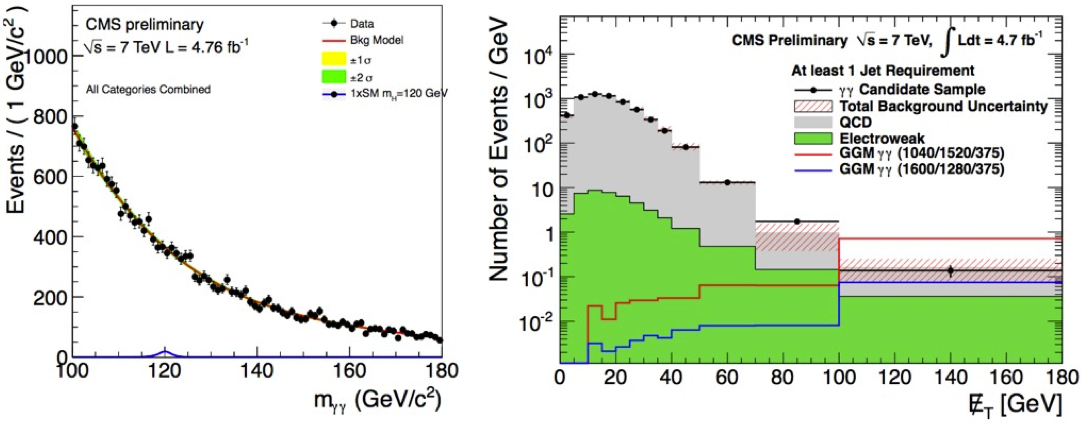
Fig. 28 Left: Higgs boson search in 2011. Right: search for an excess of events at high missing transverse energy. In both cases the data are well described by the background only hypothesis.

Neyman Pearson Lemma

We haven’t addressed up to now the choice of \(t_{cut}\). The only thing we know up to now is that it affects the efficiency and the purity of the sample under study. Ideally what we want is to set the desired efficiency and for that value get the best possible purity.
Take the case of a simple hypothesis \(H_0\) and allow for an alternative simple hypothesis \(H_1\) (e.g. the typical situation of signal and background). The Neyman Pearson lemma states that the acceptance region giving the highest power (i.e. the highest purity) for a given significance level \(\alpha\), is the region of space such that:

\[\frac{g(\vec{t} | H_{0})}{g(\vec{t} | H_{1})} > c,\]

where \(c\) is the knob we can tune to achieve the desired efficiency and \(g(\vec{t}|H_{i})\) is the distribution of \(\vec{t}\) under the hypothesis \(H_{i}\).

Basically what the lemma says is that there is function \(r\) defined as

\[ \begin{aligned} r = \frac{g(\vec{t} | H_{0})}{g(\vec{t} | H_{1})}\end{aligned} \]

that brings the problem to a 1 dimensional case and that gives the best purity given a fixed efficiency. The function \(r\) is called the likelihood ratio for the simple hypotheses \(H_0\) and \(H_1\) (in the likelihood the data are fixed, the hypothesis is what is changed). The corresponding acceptance region is given by \(r>c\). Any monotonic function of \(r\) will be good too and will lead to the same test.

The main draw back of the Neyman-Pearson lemma is that is is valid if and only if both \(H_0\) and \(H_1\) are simple hypothesis (and that is pretty rare). Even in those cases in order to determine c one needs to know \(g(\textbf{t}|H_{0})\) and \(g(\textbf{t}| H_{1})\). These have to be determined by Monte Carlo simulations, or data driven techniques, for both data and background. The simplest way to represent the p.d.f.’s is to use a multidimensional histogram. This can cause some troubles when the dimensionality of the problems is high. Say we have \(M\) bins for each of the \(n\) dimension of the test statistics \(\textbf{t}\), then the total number of bins is \(M^n\), i.e. \(M^n\), parameters must be determined from Monte Carlo or data and this can quickly become impractical. We will see later (Ch. MVA) a different way to model the p.d.f. using Multi-Variate techniques.

Goodness of Fit

A typical application of hypothesis testing is to assess the goodness of a fit, i.e. quantifying how well the null hypothesis \(H_0\) describes a sample of data, without any specific reference to an alternative hypothesis. The test statistic has to be constructed such that it reflects the level of agreement between the observed data and the predictions of \(H_0\).
The typical quantitative way to assess the agreement is to use the concept of \(p-\)value. As we have already seen (Eq. (11)) the \(p-\)value is the probability, under the assumption of H, to observe data with equal or less compatibility with \(H_0\), relative to the data we got.
N.B.: the \(p-\)value does not give the probability for \(H_0\) to be true! As a frequentist the probability of the hypothesis is not even defined: the probability is defined on the data. As Bayesian the probability of the hypothesis is a different thing and it is defined through the Bayes theorem using the prior hypothesis.

The \(\chi^2\)-Test

We have already encountered the \(\chi^2\) as a goodness of fit test in section Sec.Least Squares. The \(\chi^{2}\)-test is by far the most commonly used goodness of fit test. The first application we discuss is with a set of measurements \(x_i\) and \(y_i\), where the \(x_i\) are supposed to be exact (or at least with negligible uncertainty) and the \(y_i\) are known with an uncertainty \(\sigma_i\). We want to test the function \(f(x)\) which we believe it gives (predicts) the correct value of \(y_i\) for each value of \(x_i\); to do so we define the \(\chi^2\) as:

\[\chi^{2} = \sum_{i=1}^{N} \frac{[y_{i}-f(x_{i})]^{2}}{\sigma_{i}^{2}}.\]

If the uncertainties on the \(y_i\) measurements are correlated, the above formula becomes (with the lighter matrix notation, see Sec.Matrix Notation:

\[\chi^{2} = (\bf{y}-\bf{f})^T \bf{V}^{-1} (\bf{y} - \bf{f})\]

where \(\bf{V}\) is the covariance matrix. A function that correctly describes the data will give a small difference between the values predicted by the function \(f\) and the measurements \(y_i\). This difference reflects the statistical uncertainty on the measurements, so for \(N\) measurements the \(\chi^2\) should be roughly \(N\).

Recalling the p.d.f. of the \(\chi^2\) distribution (see Sec.\(\chi^2\)):

\[ \label{Chi2EquationAgain} P(\chi^{2};N) = \frac{2^{\frac{-N}{2}}}{\Gamma\left(\frac{N}{2}\right)} \chi^{N-2} e ^{\frac{-\chi^{2}}{2}} \]

(where the expectation value of this distribution is \(N\), and so \(\chi^{2} / N \sim 1\)), we can base our decision boundary on the goodness-of-fit, by defining the \(p-\)value:

\[ \label{Chi2Probability} p = \text{Prob}(\chi^{2};N) = \int_{\chi^{2}}^{\infty} P(\chi'^{2}; N) d\chi'^{2} \]

which is called the \(\chi^{2}\) probability. This expression gives the probability that the function describing the \(N\) measured data points gives a \(\chi^{2}\) as large or larger than the one we obtained from our measurement.

Example:

Suppose you compute a \(\chi^2\) of 20 for N=5 points. The feeling is that the function is a very poor model of the data (\(20/5 =4 \gg 1\)). To quantify that we compute the \(\chi^2\) probability \(\int_{20}^{\infty}P(\chi^2,5)d\chi^2\). In ROOT FIXME you can compute this as TMath::Prob(20,5) = 0.0012. The \(\chi^2\) probability is indeed very small and the \(H_0\) hypothesis should be discarded.

You have to be careful when using the \(\chi^2\) probability to take decisions. For instance if the \(\chi^2\) is large, giving a very small \(\chi^2\) probability, it could be both that the function \(f\) is a bad representation of the data or that the uncertainties are underestimated.

Here the function is given, not fitted on data.

On the other hand if you obtain a very small value for the \(\chi^2\), the function cannot be blamed, so you might have overestimated the uncertainties. It’s up to you to interpret correctly the meaning of the probability. A very useful tool for this scope is the pull distribution (see Sec. ML remarks), where each entry is defined as (measured-predicted)/uncertainty = \((y_i - f(x_i))/ \sigma_i\); if everything is done correctly (i.e. the model is correct and the uncertainties are computed correctly) the pull will result in a normal distribution centred at 0 with width 1. If the pull is not centred at 0 (bias) the model is incorrect, if the pull has a width larger than 1 either the uncertainties are underestimated or the model is wrong, if the pull has a width smaller than 1 the uncertainties are overestimated.

Degrees of freedom for \(\chi^2\)-test on fitted data

The concept of \(\chi^2\) developed above only works if you are given a set of data points and a function (model). If the function comes out from a fit to the data then, by construction, you will get a \(\chi^2\) which is the smallest, because you fit the parameters of the function in order to minimize it.

This problem turns out to be very easy to treat. You just need to remove degrees of freedom from the computation. For example, suppose you have \(N\) points and you fitted \(m\) parameters of your function to minimize the \(\chi^2\) sum; then all you have to do to compute the new \(\chi^2\) probability is to reduce the number of d.o.f. to \(n=N-m\).

Example:

You have a set of 20 points, you consider as function f(x) a straight line and you get \(\chi^2 = 36.3\). If you use a parabola you get \(\chi^2 = 20.1\). The straight line has 2 degrees of freedom (slope and intercept), so the number of d.o.f. of the problem is 20-2=18; the \(\chi^2\) probability is FIXME TMath::Prob(36.3,18) = 0.0065 which makes the hypothesis that data are described by a straight line improbable. If you now fit it with a parabola you get TMath::Prob(20.1,17) = 0.27 which means that you can’t reject the hypothesis that the data are distributed according to a parabolic shape.

Notes on the \(\chi^{2}\)-test:

• For large values of d.o.f. the distribution of \(\sqrt{2\chi^2}\) can be approximated with a Gaussian distribution with mean \(\sqrt{2n-1}\) and standard deviation \(1\). When in the past the integrals were extracted from tables this was a neat trick; still it is a useful simplification when the the \(\chi^2\) is used in some explicit calculation.

• The \(\chi^{2}\)-test can also be used as a goodness of fit test for binned data. The number of events in bin \(i\) (\(i = 1, 2, \ldots, n\)) are \(y_{i}\), with bin \(i\) having mean value \(x_{i}\). The predicted number of events is thus \(f(x_{i})\). The errors are given by Poisson statistics in the bin (\(\sqrt{f(x_i)}\), see Ch. Binned \(\chi^2\) for the use of the Poisson uncertainties) and the \(\chi^{2}\) is

  \[\chi^{2} = \sum_{i=1}^{n}\frac{[y_{i}-f(x_{i})]^{2}}{f(x_{i})},\]

  where the number of degrees of freedom \(n\) is given by the number of bins minus the number of fitted parameters (do not forget the overall normalization of the model when counting the number of fitted parameters).

• when binning data, you should try to have enough entries per bin such that the computation of the \(\chi^2\) is actually meaningful; as a rule of thumb you should have at least 5 entries per bin. Most of the results for binned data are only true asymptotically.

Unbinned tests

Unbinned tests are used when the binning procedure would result in a too large loss of information (e.g. when the data set is small).

They are all based on the comparison of the cumulative distribution function (c.d.f.) \(F(x)\) of the model \(f(x)\) under some hypothesis \(H_0\) and the c.d.f. for the data. To define a c.d.f. on data we define an order statistics, i.e. a rule to order the data and then define on it the Empirical Cumulative Distribution Function e.c.d.f.:

\[\begin{split}S_n(x) = \left\{ \begin{array}{rll} 0 &\mbox{,} & x <x_1 \\ \frac{r}{n} &\mbox{,} & x_r \le x < x_{r+1} \\ 1 &\mbox{,} & x_n <x \end{array} \right.\end{split}\]

This is just the fraction of events not exceeding x (which is a staircase function from 0 to 1), see Fig. 29

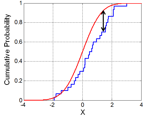
Fig. 29 Example of c.d.f. and e.c.d.f.. The arrow indicates the largest distance used by the Kolmogorov-Smirnov test.

The first unbinned test we describe is the Smirnov-Cramér-von Mises test. We define a measure of the distance between \(S_n(x)\) and F(x) as:

\[W^2 = \int_0^1 [S_n(x) - F(x)]^2 dF(x)\]

(dF(x) can be in general a non decreasing weight). Inserting the explicit expression of \(S_n(x)\) in this definition we get:

\[nW^2 = \frac{1}{12n} + \sum_{i=1}^n \left( F(x_i) - \frac{2i-1}{2n} \right)^2\]

From the asymptotic distribution of \(nW^2\) the critical regions can be computed: frequently used test sizes are given in the Tab. Fig. 30. The asymptotic distribution is reached remarkably rapidly (in this table the asymptotic limit is reached for \(n \ge 3\)).

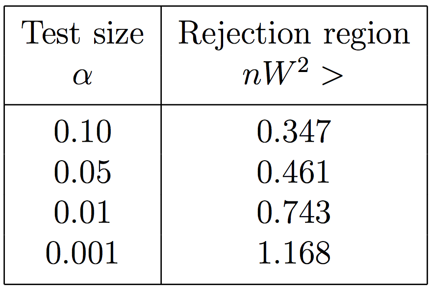
Fig. 30 Rejection regions for the Smirnov-Cramér-von Mises test the for some typical test sizes.

The Kolmogorov-Smirnov test follows the same idea of comparing the model c.d.f. with the data e.c.d.f. but it defines a different metric for the distance between the two. The test statistic is \(d := D \sqrt{N}\) where \(D\) is the maximal vertical difference between \(F_{n}(x)\) and \(F(x)\) (see Fig. 29:

\[D := \max_{x} |S_{n}(x)-F(x)|\]

The hypothesis \(H_{0}\) corresponding to the function \(f(x)\) is rejected if \(d\) is larger than a given critical value. The probability \(P(d\le t_0)\) can be calculated in FIXME ROOT by TMath::KolmogorovProb(t0). Some values are reported in Fig. 31.

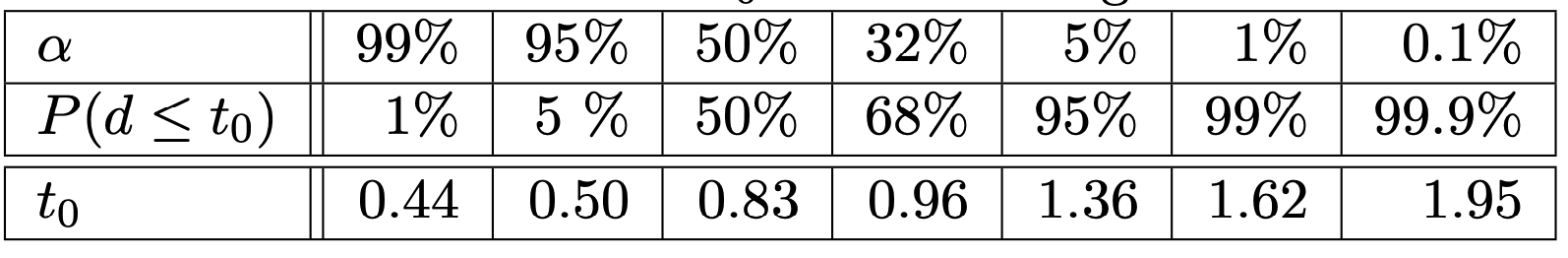
Fig. 31 Rejection regions for the Kolmogorov-Smirnov test for some typical test sizes.

The Kolmogorov-Smirnov test can also be used to test if two data sets have been drawn from the same parent distribution. Take the two histograms corresponding to the data to be compared and normalize them (such that the cumulative plateaus at 1). Then compare the e.c.d.f. for the two histograms and compute the maximum distance as before (in FIXME ROOT use h1.KolmogorovTest(h2)).

Notes on the Kolmogorov-Smirnov test:

• the test is more sensitive to departures of the data from the median of \(H_0\) than to departures from the width (more sensitive to the core than to the tails of the distributions)

• the test becomes meaningless if the \(H_0\) p.d.f. is a fit to the data. This is due to the fact that there is no equivalent of the number of degrees of freedom as in the \(\chi^{2}\)-test, hence it cannot be corrected for.

Two-sample problem

In this section we will look at the problem of telling if two samples are compatible with each other, i.e. if both are drawn from the same parent distribution. Clearly the complication is that, even if they are, they will exhibit differences coming from statistical fluctuations. In the following we will examine some typical examples of two-sample problems (see Fig. 33).

Two Gaussians, known \(\sigma\)

Suppose you have two random variables \(X\) and \(Y\) distributed as Gaussians of known width. Typical situations are when you have two measurements taken with the same device with a known resolution; or two samples are taken under different conditions where the variances of the parent distribution are known (you have the two means \(\langle X \rangle\), \(\langle Y \rangle\) and the uncertainty on the means \(\sigma_x/\sqrt{N_x}\) and \(\sigma_y/\sqrt{N_y}\)).

This problem is equivalent to check if \(X-Y\) is compatible with \(0\). The variance of \(X-Y\) is \(V(X-Y) = \sigma_x^2 +\sigma_y^2\) and so the problem boils down to how many \(\sigma\) the difference is from 0: \((X-Y)/ \sqrt{\sigma_x^2 + \sigma_y^2}\).

More generally what you are doing is defining a test statistics \(\frac{|\langle x \rangle - \mu_0|}{\sigma/\sqrt{N}}\) (in the previous case \(\mu_0 = 0\)) and a double sided rejection region. This means that you choose the significance of your test (\(\alpha\)) and set as rejection region the (symmetric) values \(u_{1-\alpha/2}\) on the corresponding Gaussian as:

\[\int_{-\infty}^{u_{1-\alpha/2}} G(x;\mu_0,\sigma)dx = \int_{u_{1-\alpha/2}}^{\infty} G(x;\mu_0,\sigma)dx = \frac{\alpha}{2}\]

If the measured difference ends up in the rejection region (either of the two tails) then the two samples are to be considered different.
You can also test whether \(X>Y\) (or \(Y>X\)). In this case the test statistic is \(\frac{(\langle x \rangle - \mu_0)}{\sigma/\sqrt{N}}\) and the rejection region becomes single sided \((u_{1-\alpha},\infty)\) (or \((-\infty,u_{1-\alpha})\)).

Two Gaussians, unknown \(\sigma\)

The problem is similar to the previous one, you’re comparing two Gaussian distributions with means \(\langle X \rangle\) and \(\langle Y \rangle\), but this time you don’t know what are the parents’ standard deviations. All you can do is to estimate them from the samples at hand:

\[s^2_x = \frac{\sum(x_i -\langle x\rangle)^2}{N_x-1} \qquad ; \qquad s^2_y = \frac{\sum(y_i -\langle y\rangle)^2}{N_y-1}.\]

Because we’re using the estimated standard deviation we have to build a Student’s \(t\) variable to test the significance, and not the Gaussian p.d.f. as we did in the previous case. As we have seen in Sec. Student’s \(t\) the \(t\)-variable comes from the ratio of a Gaussian and a \(\chi^2\) variable; the trick was to cancel out in the ratio our ignorance about \(\sigma\).

For the numerator, the expression

\[\frac{\langle x \rangle - \langle y \rangle}{\sqrt{(\sigma_x^2/N_x)+(\sigma_y^2/N_y)}}\]

under the null hypothesis that the two distributions have the same mean (\(\mu_x = \mu_y\)) is a Gaussian centred at zero with standard deviation one.

For the denominator, the sum

\[\frac{(N_x-1)s_x^2}{\sigma_x^2} + \frac{(N_y-1)s_y^2}{\sigma_y^2}\]

is a \(\chi^2\) (to convince yourself just plugin the \(s^2_x\) and \(s^2_y\) written above) with \(N_x+N_y-2\) d.o.f, because we used them to compute the means.

If we assume that the unknown parent standard deviation is the same for the two samples \(\sigma_x = \sigma_y\), that will do the trick: \(\sigma\) cancels out in the ratio. The definition for the \(t\)-distribution becomes:

\[t = \frac{\langle x \rangle - \langle y \rangle}{S \sqrt{(1/N_x)+(1/N_y)}}\]

where

\[S^2 = \frac{(N_x-1)s_x^2 + (N_y-1)s_y^2}{N_x +N_x -2}\]

The variable \(t\) is distributed as a Student’s \(t\) with \(N_x +N_x -2\) d.o.f. With this variable we can now use the same testing procedure (double or single sided rejection regions) used in the case shown above in known \(\sigma\) substituting the c.d.f of the Gaussian with the c.d.f. of the Student’s t.

F-test

The \(F\)-test is used to test whether the variances of two samples with size \(n_{1}\) and \(n_{2}\), respectively, are compatible. Because the true variances are not known, the sample variances \(V_{1}\) and \(V_{2}\) are used to build the ratio \(F = \frac{V_{1}}{V_{2}}\). Recalling the definition of the sample variance, we can write:

\[F= \frac{V_{1}}{V_{2}}=\frac{\frac{1}{n_{1}-1}\sum_{i=1}^{n_{1}}(x_{1_{i}}-\bar{x}_{1})^{2}}{\frac{1}{n_{2}-1}\sum_{i=1}^{n_{2}}(x_{2_{i}}-\bar{x}_{2})^{2}}\]

(by convention the bigger sample variance is at the numerator, such that \(F \geq 1\)). Intuitively the ratio will be close to 1 if the two variances are similar, while it will go to a large value if they are not. When you divide the variance by \(\sigma^2\) you obtain a random variable which is distributed as a \(\chi^2\) with \(N-1\) d.o.f. Given that the random variable \(F\) is the ratio of two such variables, the \(\sigma^2\) cancels and we are left with the ratio of two \(\chi^2\) distributions with \(f_1 = N_1-1\) d.o.f. for the numerator and \(f_2=N_2-1\) d.o.f. for the denominator.

The variable \(F\) follows the \(F\)-distribution with \(f_1\) and \(f_2\) degrees of freedom: \(F(f_{1},f_{2})\):

\[P(F) = \frac{\Gamma((f_1+f_2)/2)}{\Gamma(f_1/2)\Gamma(f_2/2)}\sqrt{f_1^{f_1} f_2^{f_2}}\frac{F^{f_1/2-1}}{(f_1+f_2F)^{(f_1+f_2)/2}}\]

For large numbers, the variable

\[Z= \frac{1}{2} \log{F}\]

converges to a Gaussian distribution with mean \(\frac{1}{2}(1/f_2-1/f_1)\) and variance \(\frac{1}{2}(1/f_2+1/f_1)\). In any case you can test the compatibility by using e.g. the FIXME ROOT function TMath::fdistribution_pdf.

Example:

Background model for the \(H\to \gamma\gamma\) search: The collected diphoton events are divided in several categories (based on resolution and S/B to optimize the analysis sensitivity). Once a model for the background is chosen (e.g. a polynomial) the number of d.o.f. for that model (e.g. the order of the polynomial) can be chosen using an F-test. The main idea is gradually increase the number of d.o.f. until you don’t see any decrease in the variance (see snapshot of the text here below).

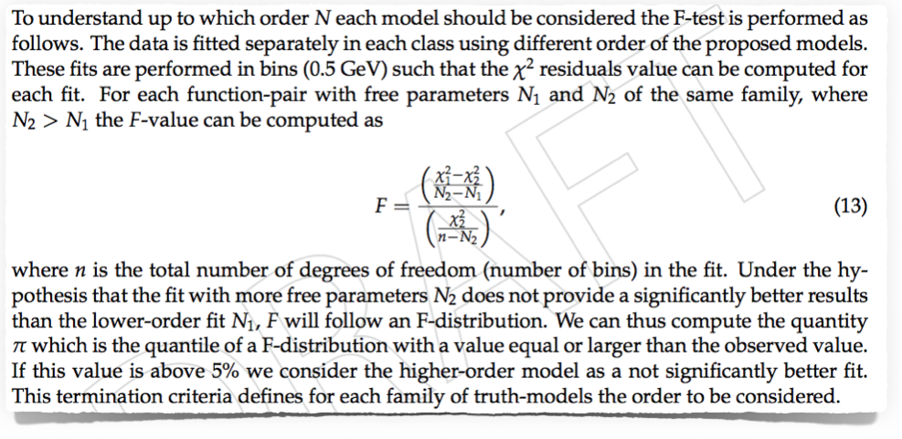
Fig. 32 Example from the CMS Hgg analysis. (FIXME find published paper text)

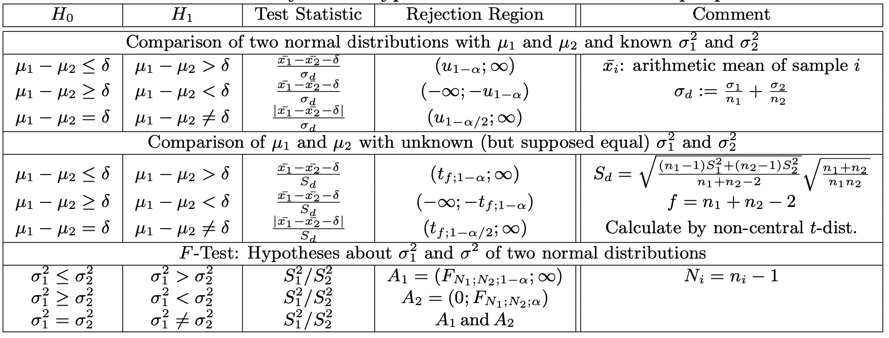
Fig. 33 Summary of the hypothesis tests for the two-sample problem.

Matched and correlated samples

In the previous sections we’ve seen how to compare two samples under different hypothesis. The tests are more discriminating the smaller are their variances. Correlations between the two samples can be used to our advantage to reduce the variance. Take as test statistic:

\[\sum_i (x_i-y_i)\]

where each of the data point of the first sample is paired to a corresponding one in the second sample. The variance of this distribution is:

\[V(x-y) = \sigma_x^2 + \sigma_y^2 - 2\rho \sigma_x \sigma_y\]

Now, if the two samples are correlated (\(\rho > 0\)) then the variance is reduced and will make the test more discriminating.

Example:

A consumer magazine is testing a widget claimed to increase fuel economy. Here are the data on seven cars are reported in Fig. 34. Is there evidence for any improvement?

If you ignore the matching, the means are \(38.6 \pm 3.0\) and \(35.6 \pm 2.3\) for the samples with and without the widget. The improvement of 3 m.p.g. is within the statistical uncertainties. Now look at the differences. Their average is 3.0. The estimated standard deviation s is 3.6, so the error on the estimated average is \(3.6/ \sqrt{7} = 1.3\), and t is \(3.6/1.3 = 2.0\). This is significant at the 5% level using Student’s t (one-tailed test, 6 degrees of freedom, \(t_{critic}= 1.943\)).

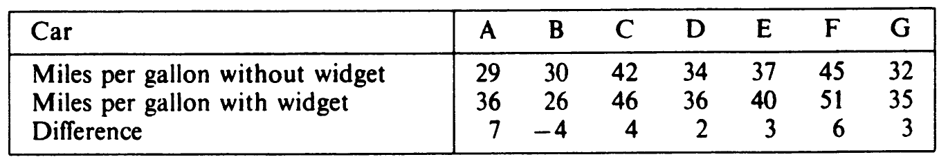
Fig. 34 Data from seven cars.

The most general test

As we already said the more precisely the test can be formulated, the more discriminant it will be. The most general two-sample test, makes no assumptions at all on the two distributions, it just asks whether the two are the same.

You can apply an unbinned test like the the Kolmogorov-Smirnov (as explained in Sec. unbinned tests by ordering the two samples and computing the maximal distance between the two e.c.d.f. Or you can approach the problem ordering together both samples and then apply a run-test. If the two samples are drawn from the same parent distribution there will be several very short runs; if on the other hand the two samples are from different parent distributions you will have long runs from both samples. This test can be tried only if he number of points in sample A is similar to the one in sample B.

Example:

Two samples A and B from the same parent distribution will give something like: \(AABBABABAABBAABABAABBBA\). Two samples from two narrow distributions with different means will give something like: \(AAAAAAAAAABBBBBBBBBBBBB\).

ANOVA

The analysis of variance (ANOVA) is a technique rarely used in high energy physics, but because of its use in natural sciences a brief introduction will be given.

The idea is a generalization of the two sample problem: instead of two samples you are confronted with several. The obvious approach to compare the different samples in pairs doesn’t work. Suppose as an example that you have 15 samples and you have to decide if they are sampled from the same parent distribution (i.e. they are “compatible”). If you start comparing them in pairs you will end up with \(\binom{15}{2}\) = 105 pairs. If you now set the significance at the 99% the probability to have all of them passing is \((1-0.01)^{105}\) = 0.348, i.e. the probability to make a type 1 error (reject the true hypothesis that they all come from the same parent distribution) is 1-0.348 = 0.652.
To expose the ANOVA method we take the simple case where all samples (“groups” as they are generally called in ANOVA) are Gaussian of the same unknown variance and we want to check if their means are compatible with the hypothesis of being all samples taken from the same parent distribution.
To fix the notation we set \((\mu,\sigma)\) the true mean and width of the parent distribution; \(n\) the number of groups \(g\) each with a number of events \(N_g\) and mean and variance \((\bar{x}_g,V_g)\) and true (unknown) sample mean \(\mu_g\). The total number of events is \(N\) and the mean and variance of the sample made summing together all groups are \((\bar{x},V)\).
The null hypothesis we want to test is \(H_0\) all groups are compatible (all \(\mu_g\) are the same and equal to \(\mu\)), the alternative hypothesis \(H_1\) is that there are differences.
To test if the groups are compatible means that we will have to say whether the variations we see from one group to the other are just statistical fluctuations or they are indeed the expression of coming from different parent distributions. Let’s define the “spread between the groups” as the spread of their means \(\bar{x_g}\) which follows the \(\sigma\) of the parent distribution. Clearly we don’t know \(\sigma\) but it can be estimated from the data itself looking at the variation “within the groups”. Stated in this way the problem can be solved using the \(F-\)test we ecountered in the previous section, by comparing the variances “between” and “within” the groups:

\[F=\frac{V_b}{V_w} = \frac{between}{within}\]

The numerator, the variance between the groups, can be taken as:

\[\frac{1}{n-1} \sum_g N_g (\bar{x}_g - \bar{x})^2.\]

There are \(n-1\) degrees of freedom because the mean is taken as \(\bar{x}_g\). As for the denominator we can take the estimate of \(\sigma\) from the different groups:

\[\frac{1}{N-n}\sum_g \sum_{i\in g} (x_i - \bar{x}_g)^2\]

where \(g\) is the group and \(i\) is the element within that group.

By taking the ratio of numerator and denominator we obtain an \(F-\)test. Now we just need to set the critical value for the desidered significance level and proceed as in the \(F-\) test. Note that the ANOVA method formally reduces to the Student’s \(t\) discussed in Sec. Student’s \(t\) when you have only two samples.

Example:

As an example we take the shares of industrial, financial, and textile sectors for a particular day see {numref}(fig:anovaEx). Is there any difference in the behaviour of the different sectors ?

We can compute:

• total average: \(\bar{x}\) = 0.48

• average for group 1: \(\bar{x}_1\) = 0.25; \(\bar{x}_1 - \bar{x}\) =0.23

• average for group 2: \(\bar{x}_2\) = 0.18; \(\bar{x}_2 - \bar{x}\) =0.30

• average for group 3: \(\bar{x}_3\) = 1.5; \(\bar{x}_3 - \bar{x}\) =1.02

Computing the numerator we get \(1/2 (12\times 0.23^2 + 11 \times 0.30^2 + 6\times 1.02^2) = 3.93\). Computing the variances within the groups, for the denominator we have \((44.3 + 103.6 + 161.5) / 26 = 11.9\).

The numerator (between) is even smaller than the denominator (within), so we can say that there is no evidence for different behaviour in the different sectors. If the numerator was larger than the denominator we should have used the critical values for the \(F-\)test.

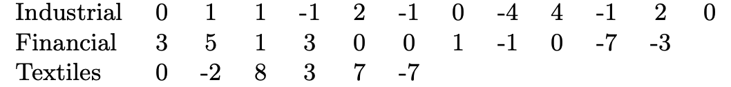
Fig. 35 The shares of industrial, financial, and textile sectors for a particular day see.

Resampling techniques

Rasampling is a technique used for non-parametric estimation of the statistical uncertainty (bias and variance) of a statistical estimator. To get an idea of non-parametric statistics see e.g. wiki. In this section we will review the two most used: jackknife and bootstrap (see B. Efron and G. Gong in References).

Non parametric techniques allow to generalize the concept of uncertainty to any estimator. Take as an example a random sample of size \(n\), \(\{ x_i\}\) with \(i=1,\ldots,n\), taken from an unknown parent distribution \(F\). Typically you will characterize the sample by computing the estimated mean and its standard deviation:

\[\bar{x} = \frac{\sum_i x_i}{n} \qquad; \qquad \hat{\sigma}=\left( \frac{1}{n-1} \sum_i (x_i - \bar{x})^2 \right)^{1/2}\]

The issue with this expression for the estimated standard deviation is that it does not generalize to any other estimator but the mean. For instance there is no way to extend it to compute the the standard deviation of the median. The resampling techniques allow to make this generalization.

Jackknife

Let’s first introduce some notation. Let

\[\bar{x}_{(i)} = \frac{n\bar{x} -x_i}{n-1} = \frac{1}{n-1}\sum_{j \neq i} x_j\]

be the average of the dataset constructed by the initial dataset, but removing the i-th element (the new sample will have n-1 elements), also known as the “deleted average”. Let

\[\bar{x}_{(\cdot)} = \sum_i \frac{\bar{x}_{(i)}}{n}\]

be the average of the sample at hand, i.e. the average of the averages computed on the samples where we have removed the i-th element (the average of the deleted averages).

The jackkinfe estimate of the standard error is defined as:

\[\bar{\sigma}_J = \left[\frac{n-1}{n} \sum_{i=1}^n (\bar{x}_{(i)} - \bar{x}_{(\cdot)})^2 \right]^{1/2}\]

which is a different way of rewriting the standard deviation, i.e.

\[\hat{\sigma} = \bar{\sigma}_J.\]

The advantage of this expression is that it can trivially be generalized to any estimator \(\hat{\theta}\) function of the \(\{x_i\}\) dataset: \(\hat{\theta} = \theta(x_1,\ldots,x_n)\). Just replace

\[\begin{split} \begin{aligned} \bar{x}_{(i)} &\to& \hat{\theta}_{(i)} = \hat{\theta}(x_1,\ldots,x_{i-1},x_{i+1},\ldots,x_n)\\ \bar{x}_{(\cdot)} &\to& \hat{\theta}_{(\cdot)} = \frac{\sum_i \hat{\theta}_{(i)}}{n} \end{aligned} \end{split}\]

The jackknife in general perform less well than the bootstrap method that we will see in the next section, but it is often preferred because computationally less expensive.

Bootstrap

The bootstrap represents a generalization of the jackknife. Again let’s start with some notation. Let \(\hat{F}\) be the empirical cumulative probability distribution function (ECDF) of the data:

\[\begin{split} \hat{F} (x) = \left\{ \begin{array}{rcl} 0 & , & x<x_{1}\\ \frac{r}{n} & , & x_{r} \leq x < x_{r+1}\\ 1 & , & x_{n} \leq x\\ \end{array} \right. \end{split}\]

and let’s define \(\{x_i^*\} = \{x_1^*, \ldots x_n^*\}\) a random sample taken from \(\hat{F}\), i.e. the \(x_i^*\) are drawn independently with repetition from \(\{x_i\} = \{x_1, \ldots x_n\}\).

For each of these samples we can compute the average and the variance:

\[\bar{x}^* = \frac{\sum_i x^*}{n} \qquad ; \qquad var_\cdot \bar{x}^* = \frac{1}{n^2} \sum_i (x_i - \bar{x})^2\]

where the dot represents the sample at hand.

As before with the jackknife this definition can be generalized to any estimator \(\bar{x}_{(\cdot)} \to \hat{\theta}_{(i)}\) as

\[\hat{\sigma}_B = \left[ var_\cdot \bar{\theta}(x_1^*,\ldots,x_n^*)\right]^{1/2}\]

and it can be verified that

\[\sqrt{\frac{n}{n-1}}~\sigma_B = \hat{\sigma}.\]

LSAT = Law School Admission Test, GPA = undergraduate Grade Point Average

To clarify the procedure let’s take the correlation coefficient \(\rho\) as an example for which we have the expression for its variance: \(\hat{\sigma} = \frac{1-\hat{\rho}^2}{\sqrt{n-3}}\). In Fig. 36 is reported a dataset made of 15 points, each representing the average LSAT and GPA scores for students coming from school \(i\) entering the american law school in 1973. This plot shows the correlation between the results of the admission exam LSAT and the average grades of undergraduate students from a school. From these data, we can estimate the sample correlation \(\hat{\rho}=0.776\) and its uncertainty \(\hat{\sigma} = 0.115\).

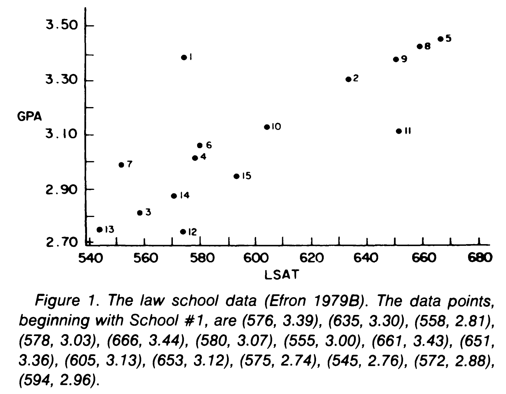
Fig. 36 Data taken from B. Efron and G. Gong in References.

Now let’s compute the sample correlation and its uncertainty using the bootstrap method writing esplicitly the algorithm.

• Build the ECDF \(\hat{F}\) on the bivariate distribution from the dataset given above.

• Draw a “bootstrap sample” \((x_1^*,\ldots,x_n^*)\), i.e. take \(n\) random draws with repetition from \((x_1,\ldots,x_n)\)

• Compute the value of the statistics (in this case the correlation coefficient) from the bootstrapped sample \(\hat{\rho}^* = \hat{\rho}(x_1^*,\ldots,x_n^*)\)

• Repeat steps 2) and 3) a large number of times \(B\) obtaining \(B\) estimations of the correlation coefficient: \(\hat{\rho}^{*1}, \hat{\rho}^{*2},\ldots,\hat{\rho}^{*B}\)

• Finally compute \(\hat{\sigma}_B = \left( \sum_{b=1}^B(\hat{\rho}^{*b} - \hat{\rho}^{*\cdot} )^2/(B-1) \right)^{1/2}\); where \(\hat{\rho}^{*\cdot} = \frac{\sum \hat{\rho}^{*b}}{B}\)

Fig. 37 shows the ditribution of \(\hat{\rho}^* - \hat{\rho}\), i.e. \(\hat{\rho}^* -0.776\) the residual between the bootstrapped estimations and the \(\rho\) computed on the dataset, using the esplicit formula. The plot has been obtained using \(B = 1000\), i.e. computing \(\hat{\rho}^{*1}, \hat{\rho}^{*2},\ldots,\hat{\rho}^{*1000}\). Using the algorithm above we obtained \(\hat{\sigma}_B = 0.127\) to be compared with the \(\hat{\sigma} = 0.115\).

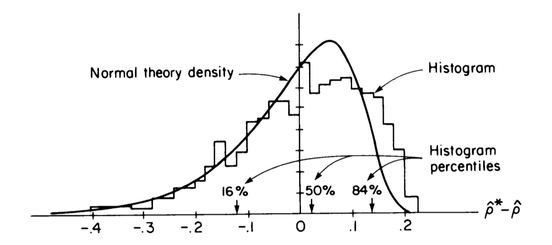
Fig. 37 Histogram of \(B=1000\) bootstrap replication of \(\hat{\rho}^*\) for the law school data. The normal theory density curve is overlapped.

Another application of the resampling techniques is the estimation of the bias (this is what the resampling was originally designed for). Let \(\hat{\theta} = \theta(\hat{F})\) and define the bias \(\beta = E[\theta(\hat{F}) - \theta(F)]\), where F is the unknown parent distribution and \(\hat{F}\) is the sampled distribution. We can consider the bias just as another estimator and so we “bootstrap the bias” i.e. compute the bootstrap estimate of the bias.

\[\hat{\beta}_B = \beta(\hat{F}) = E_*[\theta(\hat{F}^*) - \theta(\hat{F})]\]

where \(E_*\) is the expectation value on the bootstrap sampling and \(\hat{F}^*\) is the ECDF of the bootstrapped sample.
\(\beta_B\) is computed with the same algorithm we used before to compute \(\sigma_B\):

\[\beta_B = \hat{\theta}^{*\cdot} - \hat{\theta} = \frac{1}{B}\sum_{b=1}^B (\hat{\theta}^{*\cdot} - \hat{\theta})\]

Example:

A common application of the resampling techniques is when you apply two different estimators of the same parameter to the dataset at hand and you ask yourself if the two estimates are compatible. We will follow an example from literature [@jackknifeHgg].
The estimates of the best fit of the signal strength modifier of the Higgs decaying into two photons are: for the first method \(0.54^{+0.31}_{-0.26}\) for the second \(0.96^{+0.37}_{-0.33}\).

Fig. 38 is the excerpt from the paper discussing the compatibility.

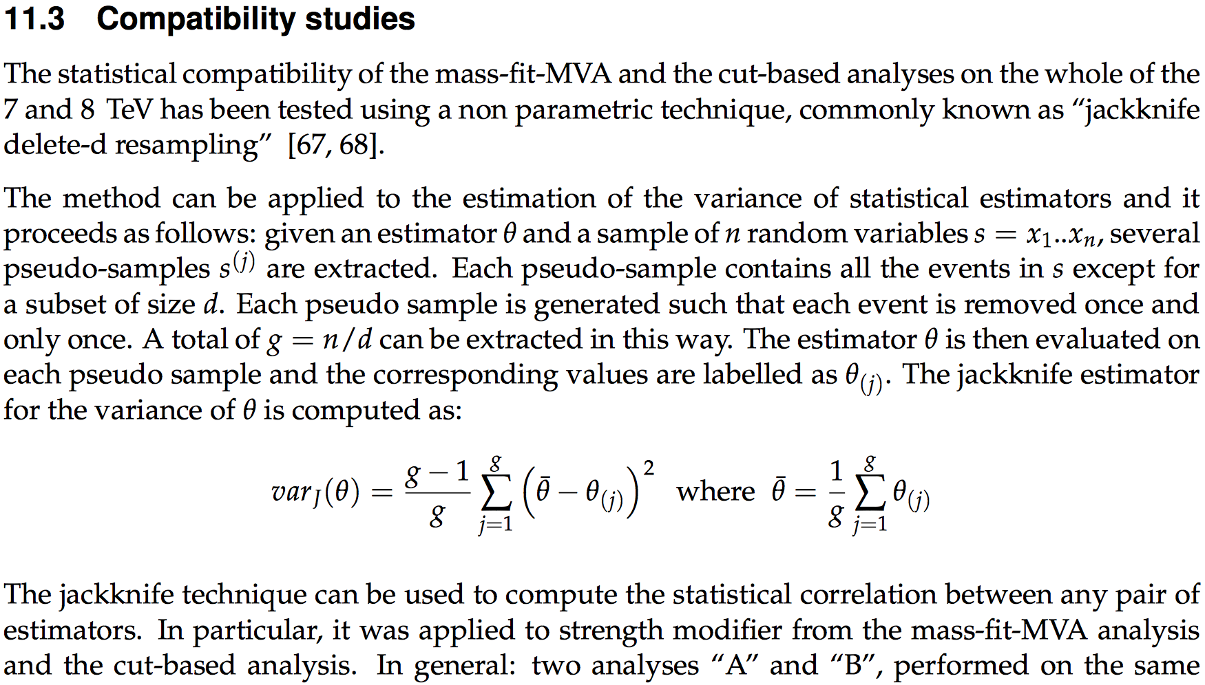
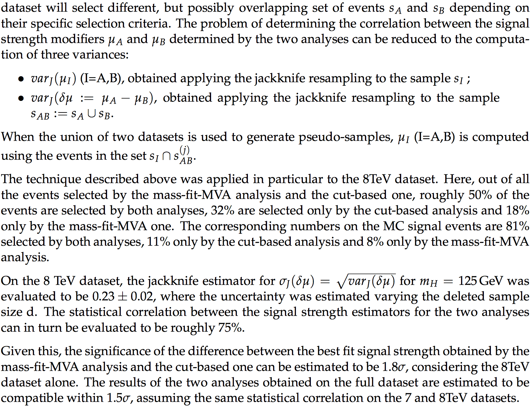
Fig. 38 \(H\to\gamma\gamma\) compatibility studies.

Information theory to quantify the compatibility between distributions

In several real life problems, you will need to assess the compatibility between two distributions in a phase space with a large number of dimensions. To do this you can use a few metrics, coming from Information Theory.

Kullback-Leibler divergence

The Kullback-Leibler (KL) divergence tells how one probability distribution P is different from a reference one Q:

discrete case: \( D_{KL}(P||Q) = \sum_{x\in X} P(x) ~\log \left( \frac{P(x)}{Q(x)} \right) \)

continuous case: \( D_{KL}(P||Q) = \int_{-\infty}^{\infty} p(x) ~\log \left( \frac{p(x)}{q(x)} \right)dx \)

It’s defined as the expectation value of the logarithmic difference between P(x) and Q(x) (i.e. the relative entropy) Remember: entropy \(H(X) = -\sum_{x\in X}p(x)~\log p(x)\).

It can be viewed as a distance between the two distributions or the information gain when comparing two statistical models.

NB: it’s not symmetric! \( D_{KL}(Q||P) = - \sum_{x\in X} P(x) ~\log \left( \frac{Q(x)}{P(x)} \right)\)

Link to the Neyman-Pearson lemma: the best test statistics to distinguish between two distributions is the ratio of their likelihoods. The KL divergence is the expected value of this statistic.

The KL-divergence is non negative and zero when the two distributions have the same amount of information. (when \( p(x) = 0 \), \(D_{KL} = 0\) because \(\lim_{x\to 0^+} x\log(x) = 0\)).

You can find a basic numerical example here: https://en.wikipedia.org/wiki/Kullback-Leibler_divergence#Basic_example

Cross Entropy

When working with the loss function of a ML algortithm you often encounter the Cross Entropy. The Cross Entropy is closely related to the KL divergence and it is defined as:

\( H(P,Q) = H(P) - D_{KL}(P||Q)\)

i.e. it’s the same as the KL divergence without the P log P term:

\(H(P,Q) = - \sum_{x\in X} P(x) ~\log Q(x)\)

Minimising the cross entropy wrt Q = minimising the KL divergence.

Mutual Information

The mutual information of two random variables X, Y can be seen as a “generalisation of the linear correlation coefficient”. It quantifies the difference between the joint distribution P(X,Y) and the product of the marginal distributions P(X)P(Y).

Let (X,Y) two random variables: \( MI(X,Y) = D_{KL}(P(X,Y) || P(X)P(Y)) \)

MI is zero when the joint distribution coincides with the product of the marginal distributions (i.e. when X and Y are independent)

Wasserstein distance / Earth mover’s distance

The p-Wasserstein distance is defined as:

\( W_p(P,Q) = \left(\frac{1}{n} \sum_{i=1}^{n} | X_{(i)} - Y_{(i)}|^p \right)^{1/p} \)

Intuitively: each distribution is viewed as a unit amount of earth, piled on, the metric is the minimum “cost” of turning one pile into the other, which is assumed to be the amount of earth that needs to be moved times the mean distance it has to be moved.

A simple example comparing the KL-divergence with the Wasserstein distance can be found here: https://stats.stackexchange.com/questions/295617/what-is-the-advantages-of-wasserstein-metric-compared-to-kullback-leibler-diverg

References

Most of the material of this section is taken from:

• G. Cowan, [Cow98], “Statistical Data Analysis”,Ch. 4

• R. Barlow, [Bar89], “ A guide to the use of statistical methods in the physical sciences”. Ch. 8

• W. Metzger, [Met02], “Statistical Methods in Data Analysis”: Ch.10

• B. Efron and G. Gong, [EG83], “A Leisurely Look at the Bootstrap, the Jackknife, and Cross-Validation

• CMS collaboration, [CMS13b]”Updated measurements of the Higgs boson at 125 GeV in the two photon decay channel”