Multivariate Analysis Methods#
In this chapter we will describe some multi-variate analysis (MVA) methods that are very frequently used in particle physics. To put things in context the methods we will discuss belongs to the much wider area of Artificial Intelligence (AI). AI studies the systems that perceive the environment. Within this huge field, machine learning (ML) is the technology of getting computers to act without being explicitly programmed to do so. Typically we then distinguish supervised learning from unsupervised learning. In supervised learning you instruct an algorithm by examples: data are presented to the algorithm with a tag and the algorithm learns how to associate data to the different tags by analysing their characteristics. In unsupervised learning (a.k.a. clustering algorithms) the algorithm will discover by itself the different tags (populations) in data by looking at their characteristics.
In today’s HEP, supervised learning is by far the most used type of learning. These algorithms are used to solve two classes of problems: classification and regression. In a classification problem the goal is to subdivide the elements of a dataset into a discrete set of classes depending on their characteristics. Typical examples are signal/background separation or particle identification: photon/jets, etc… A regression problem is conceptually identical but the classes instead of belonging to a discrete set are represented by a continuum. Most commonly is used to improve energy measurements resolution. The reconstructed energy of a jet is affected by several detector effects which depend on the position of the jet in the detector, its shape, the reconstructed energy, etc… The regression algorithm assigns the jet to a continuous value, its “regressed energy”. It does it by looking at the examples he has been trained on and recognizing which (true) energy is closer to the case at hand.
The key point of these algorithms is that they learn from a training set of data and then they use the acquired knowledge to take decisions on data they have never seen before.
MVA techniques are coded in several packages. The most used in HEP is
TMVA FIXME [@TMVA] that comes with ROOT. Other packages often used are
scikit FIXME [@scikit] in python and R FIXME [@R].
Definitions#
In this section we will set the language that we will use to study the MVAs. We will build on the concept of test statistics developed in the previous chapters and so we conveniently use the language of statistics (we could have chosen to use the ML - computer science language, it’s just a different naming, the concepts are the same).
Let’s take as a working example a classification problem with only two classes (we will address the regression case later). In the language of statistics, implementing a classifier means to choose a decision boundary that allows to separate the two classes. To do so we characterize each event with a number of variables \(\vec{x} = (x_1,x_2, \ldots, x_n)\) and define the decision boundary as a hyper-surface in this \(n\)-dimensional space \(y(\vec{x})=c\). The function \(y(\vec{x})\) is our test statistic which compresses the full information contained in the \(n\) variables into one number.
Example:
As an example imagine you have to separate tracks into muon and electron candidates. The variables \(\vec{x}\) could be \(p_T\), \(\eta\), \(\phi\), some PID on the track, number of hits in the muon chamber, presence of an electromagnetic cluster in the same direction of the track, etc… The muon candidates will preferentially populate a certain region of this multidimensional space (e.g. large number of hits in the muon chambers) while the electrons a different one (energy deposits in the electromagnetic calorimeter). Formally the distribution of \(\vec{x}\) will follow some n-dimensional joint p.d.f. depending on the hypothesis (muon/electron): pdf\((\vec{x}|H_i), \; i= \mu, e\).
The choice of the boundary depends on several factors. It depends on the variables you choose (physics driven), on the type of classifier you want to use, on computational issues (CPU, memory) and typically it boils down to finding a compromise between performance and complexity of the classifier.
Example:
Looking at Fig. 86 we have two variables and two classes “red” and “blue” distributed according to different pdfs. The different pictures show different choices of decision boundary: (left) just a cut on each of the variables , (middle) a linear combination of the two variables (right) a non linear combination of the two variables [Gle08].
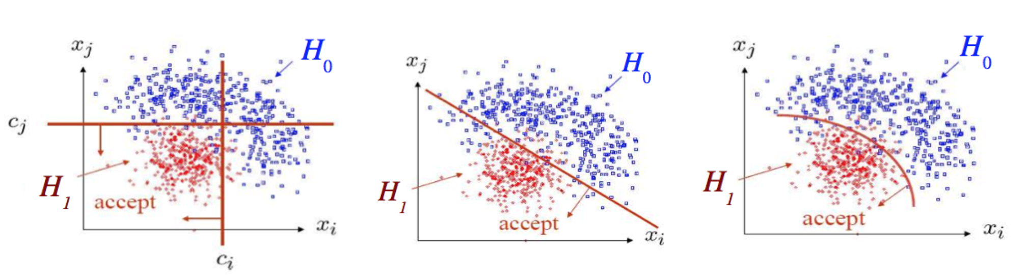
Fig. 86 Different choices of decision boundaries.#
Build the decision boundary#
For the present discussion on classification, signal and background are any two generic classes (photons/jets, jets/b-jets, cats/dogs), for simplicity we will keep calling them signal and background throughout this section.
We’ve seen in Sec.Neyman-Pearson that the optimal way to set the decision boundary having the highest background rejection for a given signal efficiency for a simple hypothesis is to use the likelihood ratio:
Unfortunately, in any non trivial practical case, we don’t have an analytic expressions for the pdf of the two classes and typically we recur to Monte Carlo techniques to model the pdfs. In this section we will see a few methods to build the pdf from Monte Carlo and see why in practice they are not used for problems with a large number of dimensions.
Histogramming#
The easiest way to build the pdf for signal and background from a Monte Carlo sample is to fill two \(n-\)dimensional histograms. This method has the advantage of being trivial to implement, and being computationally very light: the information is binned into the histogram once and then the original dataset can be discarded. The drawback of this approach is the generic problem of all histograms: need to choose a proper binning (not to coarse, not too fine) and the unavoidable discontinuities at the bin boundaries.
Kernel Density Estimators (KDE) and K-Nearest Neighbors (KNN)#
With these methods we build the decision boundary “event-by-event” judging if an event of the n-dimensional space of the variables is to be assigned to the signal region or to the background region. Intuitively, given a point \(\vec{x}\) in the n-dimensional space of the variables we count how many signal and background events are present in a local region around \(\vec{x}\) and then we apply a simple majority vote: that portion of the space is assigned to signal or background depending on which of the two has the largest population. The use of the concept of locality requires the definition of a metric in the \(n\)-dimensional space. The choice of the metric requires special consideration because the different dimensions might have different units and scales (\(E\in[10,500]\) GeV, \(\eta\in[-2.5,2.5]\), \(PID\in[0,10]\) MeV/cm, etc…). Often the variables are rescaled or remapped to have comparable numerical values in all dimensions.
Both Kernel Density Estimators (KDE) and K-Nearest Neighbors (KNN) are built around the estimator:
where \(\vec{x}\) is the point of the space we’re sampling, N is the total number of events in the sample and \(K\) is the number of events in the hyper-volume \(V\).
To optimize the classifier performance you can:
fix \(K\) and determine \(V\) \(\to\) KNN
fix \(V\) and determine \(K\) \(\to\) KDE
For the KNN you fix the number of events \(K\) (a.k.a. smoothing parameter) you want to have in your region of the space and you increase the volume \(V\) until it contains such number. Then you perform the majority vote: you count how many events are of type signal, how many are of type background and the class that has the largest number defines whether that portion of space is to be assigned to signal or background.
For the KDE you fix the hyper-volume \(V\) and change the number of events K. The “shape” for the hyper-volume \(V\) is typically chosen to be a gaussian in \(n-\)dimensions. This allows to have a smooth function for the model. (An hyper-cube would do but it would introduce discontinuities at the edges). In practice you place a gaussian kernel of standard deviation \(h\) centred about each data point, then for a given \(\vec{x}\) you add up the contribution from all the gaussians and you normalize (divide by N):
Training, bias and variance#
The classification methods shown so far use a dataset with labelled data (signal or background) to build the decision boundary. We will then use this boundary to classify new data. This procedure is called “supervised learning”; the building of the boundary is called training step while the use of the boundary is usually called application (or simply classification) step. The important point to notice is that the classifier is tuned on a sample of labelled data representative of the parent distribution of the classes, but it will be applied on new data coming from a separate sampling. Clearly, even if the training sample and the new data come from a sampling of the same distribution, they will be affected by statistical fluctuations. The training phase can reduce the mis-classification rate to zero on the training sample itself, but it will have poor performance when applied to new data.
The training has to be optimized minimizing two competing effects, the “bias-variance” tradeoff:
bias (mis-classification): the fraction of signal events ending up in the background region (or viceversa)
variance (over-training) limitation in the generalization of the classifier to different data samples
In general all methods have one or more parameters that can be tuned to find the optimal classifier. The KNN and the KDE methods have a “smoothing parameter”: \(K\) for the KNN method and \(h\) for the KDE. By tuning this parameter we can optimize our classifier. Having a large value of the smoothing parameter will produce well populated regions, reducing the statistical fluctuation, but generally increasing the bias; viceversa you can reduce the value of the smoothing parameter bringing to zero the bias but increasing the variance, i.e. making the training very sensitive to the specific sample used for training and limiting its generalization.
Curse of dimensionality and learning algorithms#
All methods described above (histogramming, KDE and KNN) become unmanageable when using a large number of input variables (dimensions). This problem goes under the name of “the curse of dimensionality”. To understand the issue, suppose your data are uniformly distributed in a \(D\)-dimensional unit cube. The methods above will all try to catch a fraction \(r\) of events in a small portion of space. Let’s suppose this portion of space has the shape of a hyper-cube with side \(s\) (its volume being \(s^D\)).
The fraction of the volume taken by this cube is \(r = s^D /1\) (the total space is a unit cube) and its side is simply \(s = r^{1/D}\). If you want a sampling fraction \(r=0.001\) (one per mill of the whole space) you will need different sizes \(s\) depending on the number of dimensions. For \(D=1\) \(s = 0.001\), for \(D=3\) \(s = 0.1\) which is 10% of the whole space, for \(D=30\) \(s=0.8\) which is 80% of the whole space. To properly build the estimator, you will need to have a very large training set to adequately populate all corners of the \(D\)-dimensional space
Learning algorithms will provide better ways to sample the space.
Fisher discriminant#
The Fisher discriminant approximates the likelihood ratio in (24) with a linear combination of the input dataset.
The decision boundary will be a constant in the one dimensional case, a
straight line in a 2-dimensional case and in general a \(n-1\) hyperplane
in an \(n\)-dimensional problem.
In the case of a Fisher discriminant the training phase consists in
finding the best set of weights \(\vec{w}\) which maximize the signal to
background (Fisher) separation. The separation is defined as:
where \(\tau_s, \tau_b\) and \(\Sigma_s, \Sigma_b\) are the mean and width (covariance) of the signal and background (see Fig. 87).
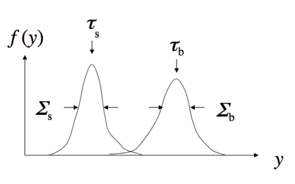
Fig. 87 Example to fix the notation in a mono-dimensional case.#
The training translates into writing the means and the covariance matrices as a linear combination of the variables and then find the weights that maximize the separation \(J(\vec{w})\). It is useful to notice that the numerator of \(J\) is the separation between the classes (the distance between the means) and the denominator is the separation within each class (the spread of the variables).
The means and covariances can be written as:
where k = “signal” or “background” and \(i,j=1,...,n\) are the components of \(\vec{x}\). From this we can compute the mean and variance of \(y(\vec{x})\)
The numerator of \(J(\vec{w})\), i.e. the separation between classes, then becomes
and the denominator
At this point we just need to maximize the ratio
by solving \(\partial J / \partial w_i = 0\). With the obtained weights we can then build the Fisher discriminant \(y(\vec{x}) = \vec{w}^T \vec{x}\).
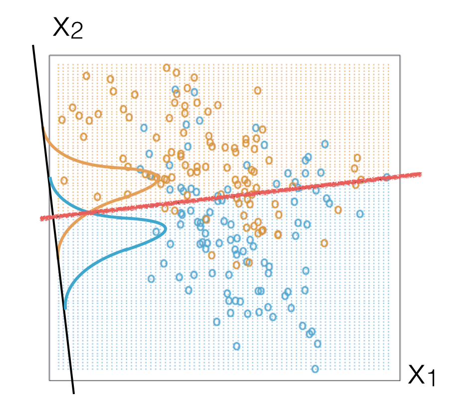
Fig. 88 Example in 2-dimensions (i.e. 2 variables). Signal is represented by orange circles, background with blue ones. The red straight line represents the Fisher discriminant which would be a linear combination of the variables \(x_1\) and \(x_2\). The orange and blue distributions visually show the separation between the projections of the two populations.#
The Fisher discriminant provides a linear decision boundary (see Fig. 88). If the classes you want to separate show some particular non linear structure like the one in Fig. 89 then you can still use a Fisher discriminant after a suitable remapping of the variables. Very often the non linear structure (especially in a multidimensional space) is not evident and for this you can use other MVA tools like BDT and ANN (see next chapters).
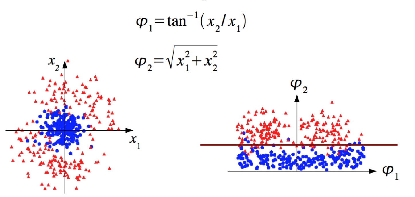
Fig. 89 The two classes show a clear symmetry: remapping them allows to still use a linear discriminant.#
Decision trees#
Because of the importance gained in recent years we will describe in some detail how to apply decision trees to solve classification and regression problems.
Classification#
A decision tree is a (binary) tree used to partition the variables’ space into rectangles and then by majority vote assign each rectangle to a class. To understand how it works we take the example in Fig. 90.
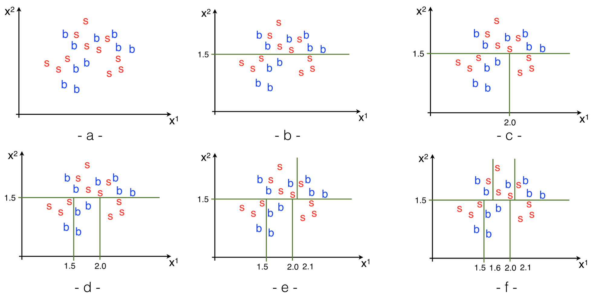
Fig. 90 Classification example.#
Let’s consider a two dimensional space (\(x^1\), \(x^2\)) and consider the usual two classes “signal” and “background” here shown in red and blue respectively as in Fig. 90-(a). In this example the variables can assume continuous values, but in reality can be any discrete or even non numerical value (an example can be a loose/tight selection criterion). To grow a decision tree means to place cuts (binary choices of the type pass/fail) to reach the minimal signal/background misclassification at each step.
The first step is to decide which variable to cut on: we choose the variable that provides the greatest increase in the separation between the two classes in the two daughters node relative to the parent. To quantify the separation we typically use as a metric the “Gini index” defined as
where the \(w_i\) are the number of signal/background events in each node (or in weights in case of weighted events). The minimal misclassification (maximal separation) is reached when \(P=0\) or \(P=1\) (selecting all signal events is equivalent to select all background events), while you get maximal misclassification (random guess, minimal separation) when \(P=0.5\). Applied to the example in Fig. 90 we will scan the two dimensions and look for the cut that maximizes the separation. In this case we select the variable \(x^2\) and a cut value of 1.5 (b). We then repeat the procedure and scan again the two dimensions to find the cut that minimizes the misclassification, this time it lead a value of 2.0 on \(x^1\). Every time we repeat the procedure we have to choose both the dimension and the value of the cut. It can happen as in (d) that the same dimension is selected twice in a raw this time cutting at 1.5. The example then continues with (e) select \(x^1\) and cut at 2.1 and (f) again selecting \(x^1\) and cutting at 1.6. The procedure will continue until we reach a minimum number of points in each of the rectangles. As we will see later in this section the minimum number of points gives a handle to limit the over-training. From the set of rectangles in Fig. 90 we can build a binary decision tree as in Fig. 91.
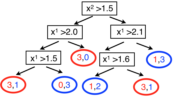
Fig. 91 Decision tree corresponding to the classification example in Fig. 90#
The last layer of the binary tree are called “leaves” (pictured as a circle) and they contain a certain number of signal and background events. In Fig. 91 they are shown as colored numbers: red for signal and blue for background. Now we have to choose how to assign each leaf to either signal or background. We do this by a majority vote. The class with the largest population defines if that leaf (or rectangle in the previous schematics) is associated with one class or the other. Again in the same figure the leaves are colored in red and blue according to the chosen class. The procedure is equivalent to writing a piece-wise constant function over the plane.
The described procedure is generally called “training”: we use labelled data (i.e. we know what is signal and what is background, as we would have with a Monte Carlo sample) and we build the tree. This is the point where the algorithm learns how to classify the data. Once this is done, we can apply the decision tree to a new dataset (never seen before by the algorithm) and use it to classify new elements. For example a point \((1.7, 1.8)\) in the previous case, would be classified as signal because it will land in the leaf/rectangle with signal=3 and background=1.
Regression#
A regression problem is conceptually equivalent to a classification one but the target variable, instead of being discrete is represented by a continuous value. In the example in Fig. 92-(a) we consider a training sample on the \(\mathbb{R}\) plane \((x,y)\).
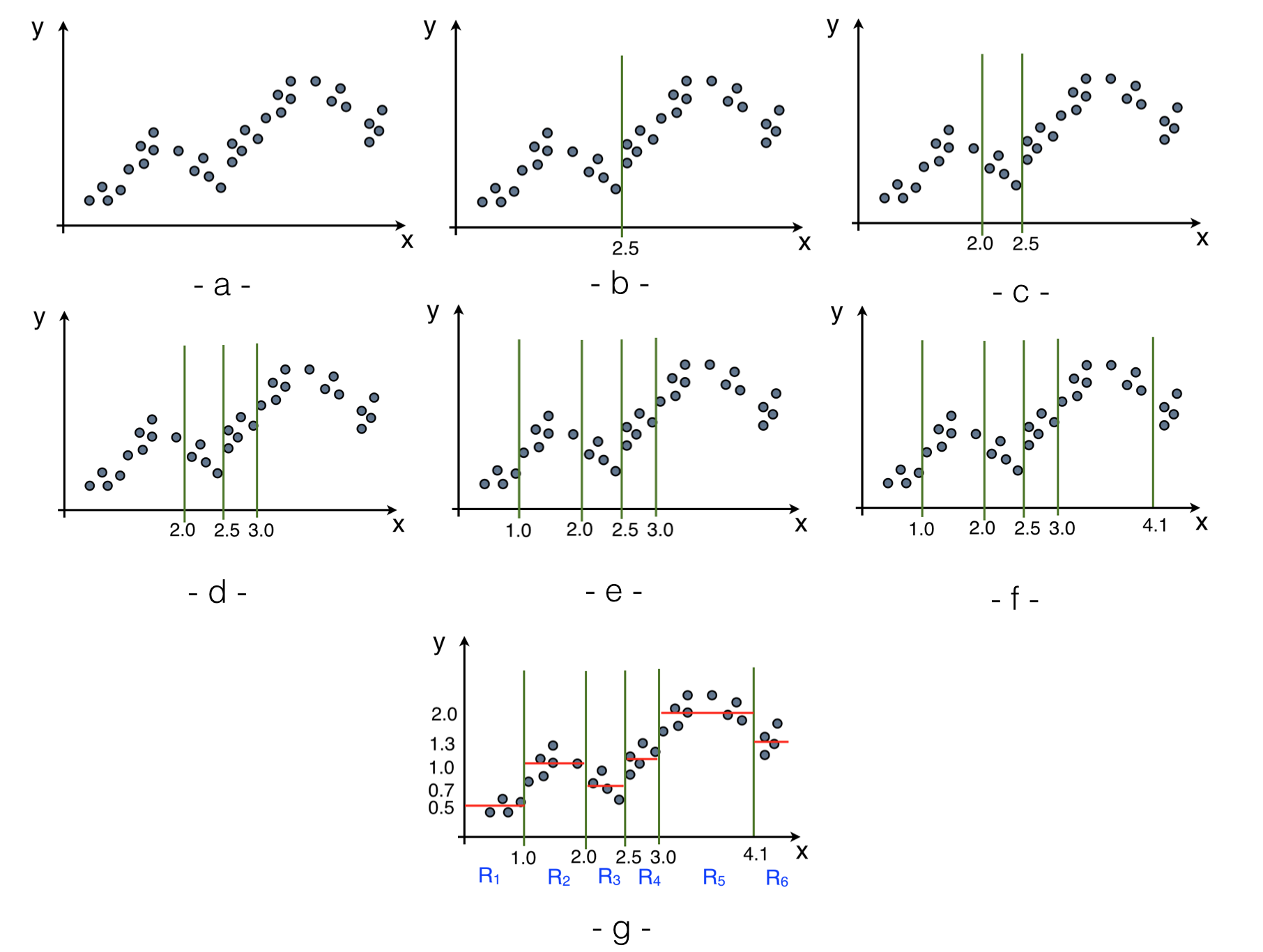
Fig. 92 Regression example.#
The idea is again the same as the one used for the classification: given a set of variables assign the correct category. Here the only difference is that the category are defined on a continuous sample. In this example the variable is \(x\) while \(y\) represent the continuous category (target). The strategy remains to set cuts such that the obtained partitions contain elements with similar characteristics (in classification we were grouping signal or background events here we group events with similar values of \(y\)). The first cut is placed at \(x=2.5\) (b) (intuitively, the left points are on average below the right ones). The we continue setting the cuts values at \(x=2.0\) (c), \(x=3.0\) (d), \(x=1.0\) (e), \(x=4.1\) (f). The procedure stops when we reach a minimum number of points in each of the regions. As in the classification case the minimum number of points gives an handle to limit the over-training. The sequence of cuts is in practice encoded in a binary tree as shown in Fig. 93. Once the regions/leaves are defined we can fit a simple model in each of them. By far the most used fit model is a simple constant ending up as in the classification case with a piece-wise constant function over the variables’ space. The values shown in the leaves of Fig. 93 represent the results of the fit to a constant shown as red lines in (g). The model used to fit the points in the final leaves can be more involved than a simple constant. If you know that the the points in the leaves will be distributed according to some principle, you can try to fit them with a parametric description of that distribution. The advantage of using a more complex model instead of a simple constant is that you will extract more information from the data (e.g. instead of just getting the mean value in a region you can extract also the width of the distribution or other parameters). To apply the regression tree we just need to take the particular point in the variables’ space we want to regress and, as in the case of the classifier, pass it through the decision tree to obtain the regressed value.
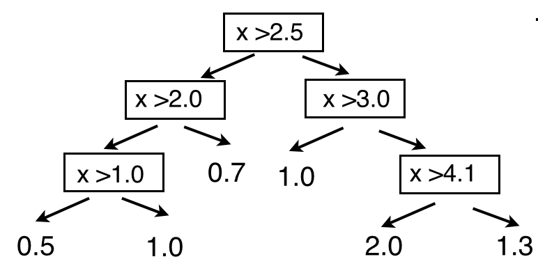
Fig. 93 Decision tree corresponding to the regression example in Fig. 92#
Stabilizing the decision trees#
Decision trees as described in the previous sections, cannot be used because are too sensitive to the particular statistical fluctuations of the training sample or in other words they have large variance. The situation changes when we apply aggregation techniques to stabilize the algorithm. The two most commonly used in HEP are “bagging” and “boosting”. In the following we will see how they work when applied to decision trees, but the aggregation methods are completely general and can be applied to any classification/regression MVA.
Bagging#
Bagging stands for Bootstrapping AGGregation. The intuition is to use a
resampling technique, the bootstrapping, shown in
Sec.Resampling
to smooth out the statistical fluctuations
of the specific training sample. We will see how it works by using as an
example the regression problem in
Fig. 94.
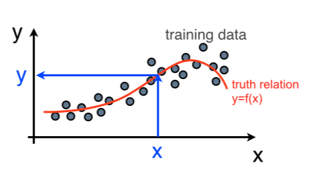
Fig. 94 Decision tree example for bagging.#
Suppose the red curve represents the truth mapping between the variables’ space and \(y\); \(y = f(x)\). The training sample, represented by the grey dots is just one sampling from the truth distribution. The Bagging technique takes N datasets independently drawn with repetition from the initial training sample, for each it builds a tree and it aggregates the resulting trees (computes the average response on the different trees).
For each of the resampled datasets \(D^i\), given a value of \(x\) we will get a regressed value of \(y(i)\). Suppose that the estimator of \(Y\) is unbiased: \(E[Y] = y = f(x)\), the variance (square distance from the true value) is \(E[(Y-y)^2] = \sigma^2(Y)\). If we define \(Z = \frac{1}{N}\sum_{i=1}^Ny(i)\), its expectation value is \(E[Z] = \frac{1}{N}\sum_{i=1}^N y = y\) and its variance is \(E[(Z-y)^2] = E[(Z-E[Z])^2] = \sigma^2(Z) = \sigma^2(\frac{1}{N}\sum_{i=1}^Ny(i)) = \left( \frac{1}{N} \right)^2 \sigma^2 (\sum_{i=1}^Ny(i)) = \frac{1}{N}\sigma^2(y)\). The larger the number of resampling the smaller the variance.
The same technique can be applied to classification problems. The only difference is that the classes instead of being defined in a continuous dataset are defined on a discrete one \(c_i \, , \, i=1, \ldots, n\) and so the numerical average over the different trees becomes a majority vote.
Boosting#
The intuition behind the boosting aggregation technique is to train several trees sequentially, each learning from the errors of the previous ones [Ihl14]. Let’s take as an example the classification problem in Fig. 95.
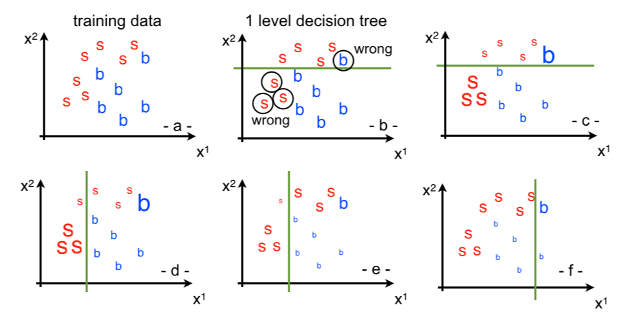
Fig. 95 Decision tree example for boosting.#
We have two variables \((x^1, x^2)\) and two classes: signal in red and background in blue (see Fig. 95 (a)). We assign a numerical value to signal and background (e.g. s = +1; b = -1), the reason for this will become clear when we will discuss the details of the boosting algorithm. In (b) we have trained a single level decision tree (which just corresponds to a single cut on the \(x^2\) variable). The tree assigns the points above the cut to signal and the ones below to background. It correctly classifies 4 signal events while it mis-classifies one background event as signal and it correctly classifies 5 background events but it mis-classifies 3 signal events as background. The idea here is to focus on the misclassified events, so we grow a second tree but this time we apply a weight to the events. We increase the weight of the misclassified and reduce the weight to the correctly classified as shown in (c); the larger/smaller events’ weights are pictured with larger/smaller fonts. Then we train a new tree like in (d). This time because of the different weights it will obviously differ from the previous one and it will find it to be more discriminating to set a cut on the \(x^1\) variable. This tree correctly classifies all the signal events below the cuts, correctly classifies six background events and mis-classifies 3 events above the cut. Repeating the procedure we increase the weights of the misclassified events and decrease the ones of the events we classified correctly as in (e). Then we train a new tree as in (f) and again repeat the procedure.
As a last step (see Fig. 96) we sum the trees we obtained with some weights which we will derive below. The regions that sum to a positive value will be assigned to signal while the ones obtaining a negative value to background. The results is that the final classifier is more complex and performant than any of the intermediate ones.
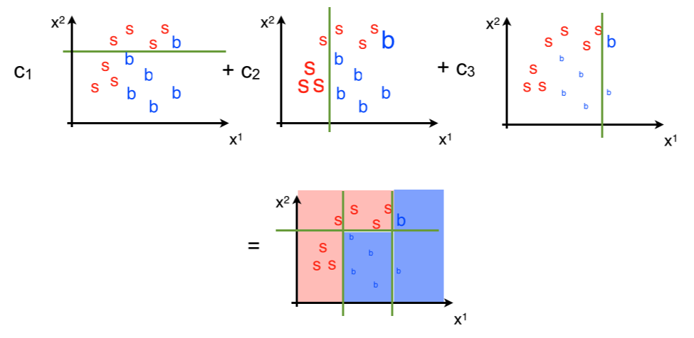
Fig. 96 Composition of the different trees.#
Back on how to set the weights. There are several different algorithms to compute the boost weights: AdaBoost, GradientBoost, etc… Here we will describe the adaptive boost (AdaBoost). The algorithm is described by the pseudo-code in Fig. 97.
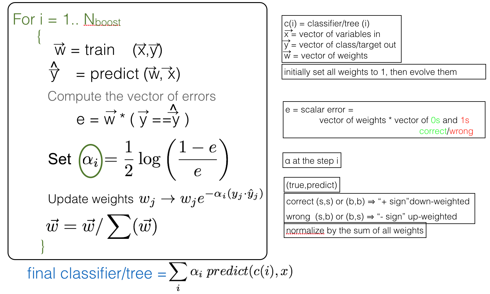
Fig. 97 AdaBoost pseudo-code.#
The algorithm starts from a uniform set of weights and it evolves them based on the mis-classifications. It starts by training a classifier (in our case a decision tree, but it could be any) based on the training sample (X,Y) and the initial set of weights (w). Then it applies the classifier to the dataset (X) obtaining a prediction \(\hat{Y}\). At this point it checks how many errors it made. It does it by producing a vector of mistakes (Y==\(\hat{Y}\) is a vector with “1” where the predicted class is correct and “0” when wrong) and taking the scalar product with the vector of weights. The result is a number “e” which represents the error rate. With this it computes \(\alpha(i)\) which is a smooth decreasing function of the error rate, for an error rate greater than 50% \(\alpha\) is negative, while it is positive for error rates below 50%). With this coefficient it computes a new vector of weights by multiplying the original one by \(w_j \to w_j \exp(-\alpha_i\cdot(Y_j\cdot\hat{Y}_j)\). At the very beginning, we assigned a numerical value of “+1” to the signal and “-1” to the background. Because of this \(Y\cdot\hat{Y}\) is a vector of “+1” and “-1”. If the predicted and the true class coincide they will have equal signs and so the product will give a “+1”, while if the prediction does not match the true value the signs will be opposite and the product give a “-1”. When multiplied by \(\alpha_i\), the weight of the correct matches will be decreased, the weight of the wrong ones increased. Finally the vector of weights is normalized. This procedure will be repeated Nboost times which is a parameter that can be optimized to get the best performance from the classifier. The final classifier is the weighted sum of all the prediction.
Artificial Neural Networks#
Artificial Neural networks (ANN or NN for short) had a large expansions in the ’80s ’90s. Then the interest in these algorithms diminished, but they are now back as the state of the art technology in machine learning (especially for classification problems) due to the enormous growth in power of modern computers (in particular through the use of GPUs). In HEP, BDT are presently dominating the scene, but it is conceivable, following the machine learning expansion, a return to neural networks in the near future.
As the name suggests, neural networks were initially inspired by the goal of producing artificial systems to simulate the functioning of a brain. In reality the structure of an artificial neural network is only loosely inspired by nature. The modelling of a basic unit (a neuron) is shown in Fig. 99.
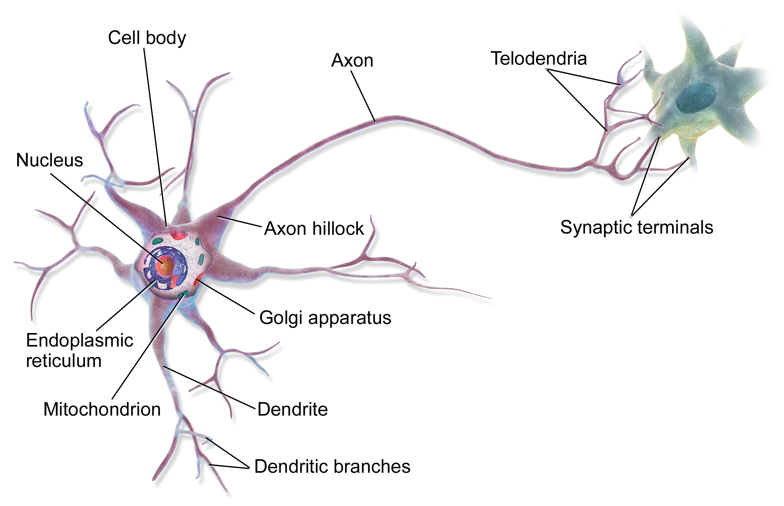
Fig. 99 Sketch of a brain cell, the neuron [wikipedia].#
A neuron receives signals through the dendrites (input wires), process them in the body of the cell (the computational unit) and outputs a signal through the axion. The axion is then connected to one of more other neurons building a network. This basic idea is replicated through software in a neural network [@Ng].
We will model a neuron as in Fig. 100. A number of inputs are fed to a computational unit which provides an output.

Fig. 100 Representation of a computational unit.#
On the left are the inputs (in this case \((x_1, x_2, x_3\))), in the centre the computational unit and on the right the output which is a function of the inputs. Conventionally the first input is \(x_1\) is fixed to “1” and it is called the bias neuron (this will simplify the vectorization of the method). The vector \(\theta\) contains all the parameters describing the neural network (called “weights”). The output function (also called activation function) is typically given by a sigmoid (but any well behaved turn-on function would do):
where \(z = \theta_{1,1}~x_1 + \theta_{1,2}~x_2 + \theta_{1,3}~x_3\) This simple neural network with just 1 layer is called single layer perceptron.
More complex networks can be put together as the one in Fig. 101.
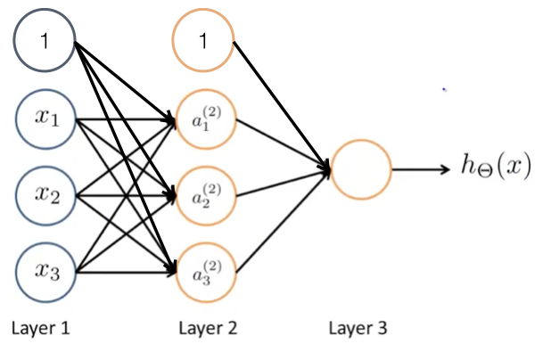
Fig. 101 Example of a neural network with one hidden layer.#
The first layer is called the input layer (Layer 1), the last layer is the output layer (Layer 3) and the layer in the midlle (which generally might be more than one) is called hidden layer. The \(a_i^{(j)}\) is the activation unit \(i\) in layer \(j\). We can translate this schematics into its corresponding mathematical expression:
where \(x_0 = 1\) a bias neuron.
Similarly, the output layer can be written as:
where \(a_0^{2} = 1\) is again a bias neuron. The process of going from the input to the output layer, performing all the computations is called forward propagation.
It is worth noting that each of the nodes of the neural network only performs a simple action on the inputs; the complexity of the final result is given by the composition of all the simple actions, i.e. by the network architechture. Another important point is that at each hidden layer, it’s the network itself which will decide what the inputs \(a_i^{(j)}\) will be. The assignment of the weights is obtained by the traning step.
The optimization of the weights \(\theta\) of the neural network is done by minimizing a cost function based on the error between the predicted classification and the true one. You can think of it as:
basically how close is the classification \(h_\theta(x^{(i)})\) to the true value \(y^{(i)}\).
The actual definition of the cost function and the algorithm to efficiently solve the minimization problem is beyond the scope of this notes (see [Ng22]. The most used algorithm is called “back-propagation” and generally speaking it finds the optimal weights by minimizing the classification error at each layer, starting from the output layer and proceding backwards to the first hidden layer.
MVA examples#
MiniBooNE [RYZ+05]was the first experiment that published an analysis based on a BDT selection. The experiment searches for neutrino oscillation and need to separate events generated by electrons, muons or neutral pions. The identification process is based on Cerenkov radiation in a tank with its inner surface covered with photomultiplier (PMT). The classifier is based on a BDT and the chosen inputs are the number of photomultiplier hits, the energy of the candidate and the radius of the reconstructed Cerenkov rings. Notice that in this case, instead of using as input variables the output of the PMTs, the information is pre-processed and “high-level” variables are instead used.
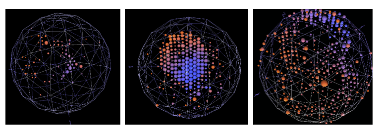
Fig. 102 Events from MiniBooNe: (left) an electron candidate, (middle) a muon candidate, (right) a \(\pi^0\) candidate.#
Another example of a classifier based on a BDT is the photon identification in the CMS \(H\to \gamma \gamma\) analysis [CMS13b]. A high energy photon is reconstructed with the electromagnetic calorimeter where it develops a narrow electromagnetic shower. A jet faking a photon is typically a jet where a light neutral meson (\(\pi^0\) or \(\eta\)) gets most of the momentum of the jet. The neutral meson decays to a photons pair but because of its boost (the analysis searches for events with high energy photons) the two photons are collimated and their showers tend to overlap in the electromagnetic calorimeter. A jet faking a photon will then appear as a shower in the electromagnetic calorimeter with a shower shape which on average will be broader than a true photon. The classifier used in CMS to separate photons from jets faking photons is based on a BDT trained on several input variables which describe the shape of the shower. The algorithm is trained on a simulated (MC) set of photons and jets. The reason why we use simulations instead of collision data is that by simulating ourself the datasets, we know how to assign unabiguously each candidate to its correct category (photon/jet).
Typically the output of a classifier will not be a binary value (“signal/background”),but a continuous value on which we will set a cut to separate the two classes. In Fig. 103 we see the output of four different classifiers applied to the same toy dataset. An easy way to compare the performance of a classifier is the “receiving operator curve” (ROC) show in Fig. 103 (bottom). This curve shows the background rejection (which is simply \(1-\epsilon_{bkg}\)) vs. the signal efficiency. The best classifier will show a curve with a sharp edge in the top right of the plot (both maximal background rejection and maximal signal efficiency). A classifier which assigns randomly events to signal and background will result in a ROC curve which is just the diagonal \(1-\epsilon_{bkg} = 1 - \epsilon_{sig}\) (i.e. \(\epsilon_{bkg} = \epsilon_{sig}\)). A standard figure of merit for to compare classifiers performance is the area under the ROC curve (AUC). In HEP the performance are often compared by fixing the efficiency at a given value (e.g. 90%) and then comparing the background rejections.
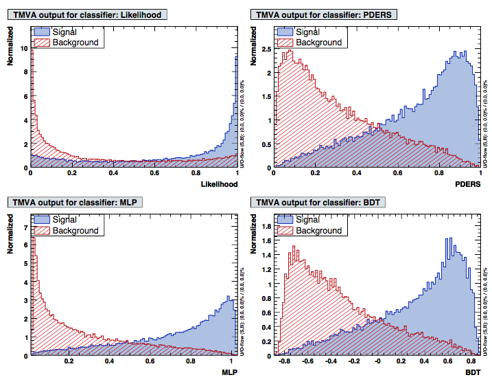
Fig. 103 Example of a classifier output (left) and the corresponding ROC curves [@TMVA].#
A typical regression problem encountered in HEP comes with energy corrections. Let’s take again as an example the energy corrections applied on electrons in CMS [CMS13a]. An electron will deposit most of its energy in the electromagnetic calorimeter. However some of it will be emitted by bremstrahlung in the material in front of the calorimeter, some in the non-instrumented gaps of the calorimeter and some might even not be correctly collected by the clustering algorithm. The regression problem consists in assigning an energy value (which is continuous, that’s why is a regression and not a classification) to the electron which is the closest to its generated energy. The algorithm is trained on a simulated (MC) sample of electrons. The reason to use simulation instead of data is to know precisely the true value of energy which is the target of the regression. The input variables chosen for the BDT are: the energy sum obtained by the clustering algorithm, several shower shape variables and the position of the electromagnetic shower in the detector. To show the effect of the regression, CMS used a sample of Z-bosons decaying to \(e^+ e^-\). The better the estimation of the energy, the better the energy resolution, the narrower is the invariance mass peak is going to be. In Fig. 104 the blue curve is the invariant mass of the \(Z\to e^+e^-\) using a very simple clustering algorithm where only the energy collected in a 5x5 matrix around the position of the electron is used; in red are the same events, this time using the CMS clustering algorithm (called “supercluster” in the legend): by better collecting the energy of the particle, the resolution on the invariant mass improves; the histogram in black shows the final improvement obtained from the energy regression described above on the electrons.
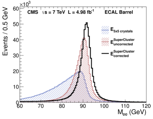
Fig. 104 Effect of the energy regression on the \(Z\to e^+ e^-\) invariant mass.#
MVAs are very commonly used also outside HEP. All major companies use them: searching suggestions, translate text, vision, voice recognition, tuning of websites advertisements, look and feel, suggestions for purchasing, etc… A simple non HEP example is the face recognition used in digital cameras. Faces are decomposed in basic features: left right symmetry, two darker shapes in the top half of the picture (the eyes), around the middle a vertical darker shape (nose) and a horizontal shape in the bottom half of the picture (the mouth). The algorithm is trained by showing a large sample of signal (faces) and background (non-faces). In Fig. 105 you can see a few examples of the classifier output applied on different pictures.
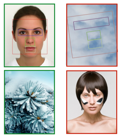
Fig. 105 Example of the output of a face recognition classifier: (top left) a face recognized as such; (top right) a cloud recognized as a face; (bottom left) pine leaves not recognized a faces; (bottom right) a face with a particular make up made to trick the face recognition algorithm.#
References#
Most of the material of this section is taken from:
Comments on BDT#
When using any MVA technique is extremely important to check for over/under-traning. Overtraining happens when the complexity of the classifier allows it to learn about the specific statistical fluctuation (noise) of the training dataset. This can be due to a traning sample too small for the number of variables used or a poorly chosen set of parameters in the algorithm training. The result of overtraining is to obtain an artificially good result in the classification/regression because the algorithms learns too many irrelevant detail of the traning sample at hand. Fig. 98 shows a classifier trained using different parameters on the same dataset.
Fig. 98 Examples of a learning algorithm trained in different ways.#
The figure on the left shows an example of overtraning. The algorithm is able to get a perfect separation between the two classes on the traning sample but it will have poor performance on a different dataset that will unavoidably have different statistical fluctuations. The middle figure shows another case of poor traning (under-training), where the algorithm complexity was not allowed to grow sufficiently. The non linearities of the training dataset are not model by the algorithm. The right picture shows an algorithm correctly trained.
A common way to check for over/under training is to split the training sample in two. On the first segment of data the “training-set”, we train the algorithm, on the second one the “test-set” (which is statistically independent from the former) we test its performance. A properly trained algorithm will show small bias and variance on both the training and the test samples.
An important characteristics of BDTs is that adding correlated variables will have little or no effect on the performance of the algorithm. The reason for this is that the best variable to cut on will be chosen at each step (based for instance on the Gini-index): any useless variable will just never be used.