Parameter Estimation - Likelihood

Take a random variable \(x\) described by a pdf \(f(x)\): the sample space is defined to be the set of all possible values of \(x\). The set of \(n\) independent measurements of the random variable \(x\), \(\{x_i\}\) is called a sample of size \(n\).

In theory of probability, from the pdf \(f(x)\) we can compute all sorts of quantities (mean, moments, etc…). In statistical inference we are concerned about the opposite problem: take the distribution of a quantity measured in data and infer its parent pdf \(f(x)\). In the simplest case of data distributed following a known pdf which depends on a parameter \(\theta\) (i.e. \(f(x,\theta)\)), the statistical inference is reduced to the extraction of the best estimate of the parameter from data.

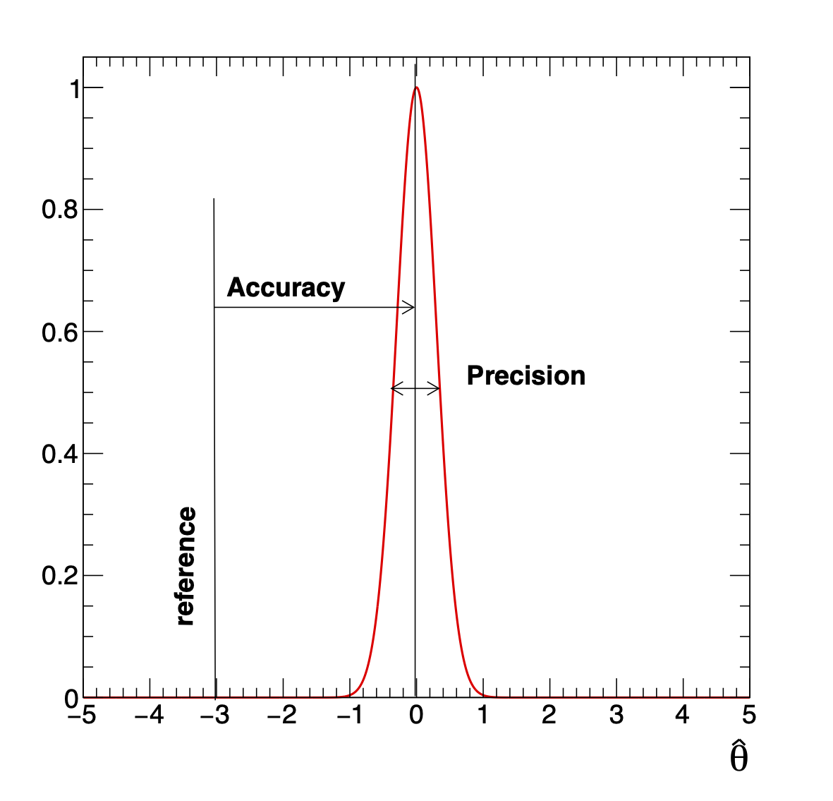
Often when talking about an estimate we use the adjectives “accurate” and “precise”. In what follows we mean (see Fig. 13):

• accuracy: how close is the estimated value to the true reference value

• precision: how reproducible the measurements are.

This means for instance that a poorly calibrated device can give you high precision but poor accuracy.

Fig. 13 Meaning of “accuracy” and “precision” Wikipedia

Any function of the observed measurements is called a statistic. A statistic used to estimate some parameter of a distribution is called estimator. We will generally denote an estimator of a parameter by adding a circumflex (\(\;\hat{ }\;\)) to the symbol of the parameter: \(\hat{\theta}\).

You can build several estimators for any parameter. As an example take the estimation of the average height of all students enrolled at ETH. Be \(h_i\) the outcome of the measurement of each of the \(N\) students, then any of the following procedures would produce an estimate:

• add all \(h_i\) and divide by N

• add only the first 15, divide by 15; ignore the rest

• add all \(h_i\) and divide by N-1

• just quote it to be 1.82 m

• multiply all \(h_i\) and take \(N^{th}\)-root of result

• choose the most popular height (mode)

• take shortest and tallest and divide by 2

• add 2\(^{nd}\), 4\(^{th}\), 6\(^{th}\),… and divide by N/2 [ or (N-1)/2 if N odd]

• take only \(h_i\) of students with brown hair, divide by M

All these are by definition estimators. Some appear to be clearly better than others, but how do we define what is a better/worse estimator? To answer this question we define some general properties of the estimators: bias, consistency, efficiency and robustness.

Properties of the estimators

The estimator \(\hat{\theta}\) being a function of random variables (data) is itself a random variable and it will be distributed according to a pdf \(g(\hat{\theta}|\theta)\), which will clearly depend on the parameter \(\theta\). We define the following properties for an estimator (see Fig. 14 )

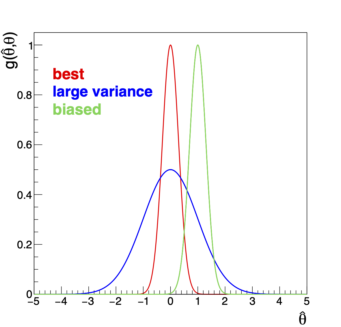
Fig. 14 Some estimator properties.

• An estimator is called unbiased if its expectation value is equal to the true value: \(<\hat{\theta}>=\theta\). Thus an estimator is biased if \(b_n = <\hat{\theta}> - \theta \ne 0\). The number \(b_n\) is called the bias of the estimator. We include the subscript \(n\) in this definition since we will see that some estimators are unbiased only asymptotically, i.e. only for \(n\to \infty\). An example of an unbiased estimator is the mean (\(\langle \bar{\mu} \rangle = \mu\)); the third in the list of the previous section is asymptotically unbiased (\(\langle \hat{\mu} \rangle = n/(n-1)\mu\)) and so \(b_n(\hat{\mu}) \to 0\) for \(n\to \infty\). If we know the bias, we can construct an unbiased estimator by correcting it.

• An estimator is called consistent if \(\forall \epsilon > 0\), \(\lim_{n \to \infty} P(|\hat{\theta}-\theta| \ge \epsilon) = 0\). For instance if \(\hat{\theta}\) is the average of data distributed according to a p.d.f. where we can apply the CLT, then \(\hat{\theta}\) is a consistent estimator because \(N(\bar{x}; \mu, \sigma^2/n)\) tends to a delta function for \(n \to \infty\). In the list of the previous section for example, the first and the third are consistent the second is not.

• An estimator is called efficient if it has the smallest possible variance of \(\hat{\theta}\) (see later in this section the minimum variance bound). The efficiency \(\epsilon\) is defined as \(\epsilon=\frac{{\rm minimal\, Variance\, of\,} \hat{\theta}}{{\rm Variance\, of\,} \hat{\theta}}\).

• An estimator is called robust if it is insensitive to wrong data or wrong assumptions, especially in the tails of a distribution.

Estimation of the Mean

The estimator for the mean \(\mu\) obtained from \(n\) independent measurements \(x_{i}\) is:

\[\label{estimate_mean} \hat{\mu}=\frac{1}{n}\sum_i x_i.\]

This estimator is unbiased, i.e. \(\langle\hat{\mu}\rangle=\langle \frac{1}{n}\sum_i x_i\rangle=\frac{1}{n}\sum_i\langle x_i\rangle = \mu\).

Furthermore it is consistent because of the CLT. Its variance is given by

\[V(\hat{\mu})=\frac{1}{n}\sigma^2.\]

Whether this estimator is efficient or not depends on the p.d.f. of the parent distribution. For instance, given a uniform distribution the mean is not the most efficient estimator; the estimator \(\hat{\mu}=0.5(x_{max}+x_{min})\) has a smaller variance. The robustness for the sample mean is increased if the truncated mean is used. This means that the largest and smallest values are trimmed (truncated). This more robust mean is less sensitive to outliers, but unless the parent distribution is symmetric it will be biased. An example for a truncated mean can be found in sports rating when only 4 out of 6 grades are used to form the final grade.

Estimation of the Variance

An estimator for the variance of a parent distribution \(\sigma^2\), when we know the true mean \(\langle x \rangle = \mu\) is:

\[ s_1^2 = \frac{1}{n}\sum_{i=1}^n (x_i - \mu)^2. \]

This estimator is unbiased

\[\begin{split} \begin{aligned} <s_1^2> &=& \frac{1}{n}\langle\sum(x_i - \mu)^2\rangle \\ &=& \frac{1}{n}\left(\langle \sum x_i^2 \rangle - 2\mu\langle \sum x_i \rangle + n \mu^2\right) \\ &=& \frac{1}{n}\left( n \langle x^2 \rangle - 2n\mu\langle x \rangle + n \mu^2\right) \qquad (independent~x_i~so~: \langle\sum x_i^2\rangle= n\langle x^2 \rangle)\\ &=& \langle x^2 \rangle - 2\mu^2 + \mu^2 \\ &=& \sigma^2 -\mu^2 + \mu^2 \qquad (\sigma^2 = \langle x^2 \rangle - \mu^2) \\ &=& \sigma^2 \\ \end{aligned} \end{split}\]

So \(s_1^2\) is an unbiased estimator of the variance of the parent p.d.f \(\sigma^2\), when \(\mu\) is known.

When it is not known, we use the estimate \(\bar{x} = \hat{\mu}\) and define:

\[ s_x^2 = \frac{1}{n}\sum(x_i-\bar{x})^2 = \bar{x^2} - \bar{x}^2 \]

The expectation value of \(s_x^2\) is:

\[ \begin{aligned} \langle s_x^2 \rangle= \frac{1}{n}\left( \langle\sum x_i^2\rangle- \frac{1}{n}\langle\left( \sum x_i \right)^2 \rangle\right).\end{aligned} \]

Substituting:

\[\begin{split} \begin{aligned} \langle\sum x_i^2\rangle&=& n\langle x^2 \rangle\\ \sigma^2 &=& \langle x^2\rangle- \mu^2\\ V\left( \sum x_i \right) &=& \langle\left( \sum x_i\right)^2\rangle- \left( \langle\sum x_i\rangle\right)^2 \end{aligned} \end{split}\]

we get

\[ \langle s_x^2\rangle= \frac{1}{n}\left( n(\sigma^2+\mu^2) - \frac{1}{n}\left( \langle\left( \sum x_i\right)^2 \rangle+ \langle\sum x_i\rangle^2 \right) \right) \]

and using

\[\begin{split} \begin{aligned} V(\langle\sum x_i\rangle) &=& \sum V(x_i) = nV(x) = n\sigma^2 \\ \langle\sum x_i\rangle&=& n \langle x \rangle= n \mu \end{aligned} \end{split}\]

we finally have

\[ \langle s_x^2 \rangle= \frac{1}{n}\left( n\sigma^2 + n \mu^2 - \frac{1}{n}(n\sigma^2 + (n\mu)^2 ) \right) = \frac{1}{n}(n-1) \sigma^2 . \]

This means that \(s_x^2\) is a biased estimator of \(\sigma^2\). The reason is that we used the sample mean \(\bar{x}\) as an estimator of the true mean \(\mu\). The spread of the data around the sample mean is less than the spread around the true mean and since the variance is the spread around the true mean \(s_x^2\) underestimates the true variance.
The formula for the variance we are used to is the one with the corrected bias:

\[ s^2 = \frac{n}{n-1} s_x^2 = \frac{n}{n-1}(<x^2> - <x>^2) = \frac{1}{n-1}\sum (x_i -<x>)^2. \]

In the same way as we got to the unbiased estimator of the variance, we obtain the expression for the unbiased estimator of the covariance \(V_{xy}\) of two random variables \(x\) and \(y\) with unknown (but estimated) means

\[ \hat{V}_{xy}=\frac{1}{n-1}\sum(x_i-<x>)(y_i-<y>)=\frac{n}{n-1}(<xy>-<x><y>). \]

The correlation coefficient is then given by

\[ \rho_{xy}=\frac{\hat{V}_{xy}}{s_xs_y}. \]

Maximum Likelihood Method

Assume we have \(n\) measurements of a random variable \(x\), distributed according to a known probability density function \(f(x|\theta)\). Where \(\theta\) stands for one parameter of the p.d.f. (e.g. the mean). Note that here you assume you know what is the correct pdf to fit and you are “only” interested in finding the value of the parameter \(\theta\) that allows the model to best fit the data.

Can we find a general method to build an estimator for \(\theta\) ( i.e. \(\hat{\theta}\) ) ? The procedure we present here goes under the name of maximum likelihood method and it is the most intuitive way to set up such an estimator.

To understand the maximum likelihood method for parameter estimation (sometimes abbreviated as ML method) we start from the probability \(f(x|\theta)dx\) (i.e. the probability to observe \(x\in (x,x+dx)\) given \(\theta\)). With this we can compute the probability to observe a certain set of data \(\{x_i\}\) given the parameter \(\theta\), as the joint probability:

\[ P= f(x_1|\theta)dx_1\cdot f(x_2|\theta)dx_2\cdot \ldots \cdot f(x_n|\theta)dx_n \]

Note that likelihood and probability are both translated in German as “Wahrscheinlichkeit”. Nevertheless there is a fundamental difference between a true analytical probability density function and a likelihood function. The latter is a function of a sample and therefore also a random variable.

The likelihood function is then defined as:

\[ L(\theta)=f(x_1|\theta)\cdot f(x_2|\theta)\cdots f(x_n|\theta)=\prod_{i = 1}^{Nevts} f(x_i|\theta). \]

where the product runs over all the events in the data sample \(\{x_i\}\) and \(L(\theta)\) is normalized to 1 for all values of \(\theta\).

The function \(L(\theta)\) is, for a given data sample, a function of only the parameter \(\theta\) and it gives us the probability to get with this choice of the parameter \(\theta\) the measured values \(\{x_{i}\}\). The likelihood function is not a probability density function in the parameters \(\theta\) (if that was the case we would calculate explicitly the expectation value of \(\theta\) and all its higher moments).

The ML principle states that the best estimate of \(\theta\) is given by the estimator \(\hat{\theta}\) which maximizes \(L(\theta)\), i.e. the value which maximizes the probability to obtain the observed set of observed data \(\{x_{i}\}\) given \(\theta\):

\[ \hat{\theta} = max_\theta~L(\theta) \]

The maximum is then computed by differentiating \(dL(\theta) / d\theta = 0\).

The concept is trivially generalized to several parameters \(a_{k}\) requiring: \(\partial L/\partial a_k=0 \ \ \forall k\).

In practice we often work with the (natural) logarithm of the likelihood function \(l(\theta) = \ln L(\theta)\) (slang: the log-likelihood). The reason for this is that likelihoods are usually calculated with computers and the product of several probabilities (i.e. numbers smaller than 1) will hit the numerical precision of the machine. The logarithm transforms the product into a sum which does not create precision problems. Since the logarithm is a monotonic rising function, the value that maximizes \(L(\theta)\) also maximizes \(\ln L(\theta)\), and our condition becomes:

\[ l(\theta)=\ln L(\theta)=\sum_{i=1}^{Nevts} \ln f(x_i|\theta) = \mbox{Maximum}. \]

Any monotonic transformation of the likelihood will leave its maximum unchanged.

It has to be stressed again that the ML estimation yields a value \(\hat{\theta}\), for which the observed data are the most “likely” (compared to other parameter values), and not vice-versa! It is not to be confused with the statement that the parameter \(\hat{\theta}\) is the most probable value.

Example:

Take the probability density given by \(f(x|\theta) = 1 + \theta(x-0.5)\) with \(x\) between 0 and 1. The provided sample data \(\{x_{i}\}= \{0.89, 0.03, 0.5, 0.36, 0.49\}\). The log-likelihood function is then given by

\[ l(\theta)=\sum_{i=1}^5 \ln(1+\theta(x_i-0.5)) \]

The maximum of the log-likelihood function can be determined graphically to be \(\hat{\theta} = -0.6\).

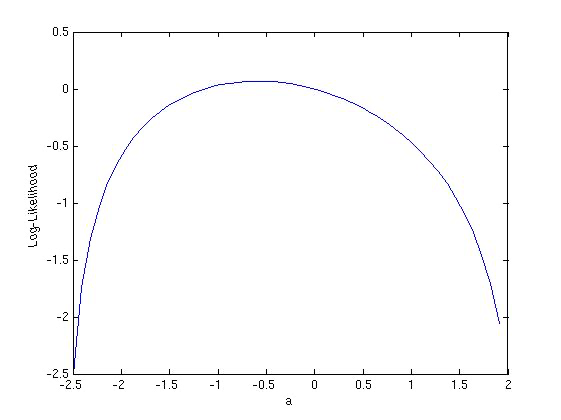
Fig. 15 The log-likelihood function from the example \(l(\theta)=\sum_{i=1}^5 \ln(1+\theta(x_i-0.5))\).

The numerical libraries in use to solve optimization problems search for minima, not maxima. To use a minimization program to find a maximum you just need to flip the sign of the likelihood: the problem is trivially moved from a maximization to a minimization. In the following we will typically work with the \(-\ln L(\theta)\) (slang: negative log-likelihood or NLL).

Example:

Exponential decay. Let’s derive the ML estimator for a particle’s lifetime. The proper decay time of an unstable particle with lifetime \(\tau\) follows the exponential distribution:

\[ f(t;\tau)=\frac{1}{\tau}e^{-t/\tau} \]

Given a set of \(n\) measurements \(\{t_i\}\) of the proper-decay time, we can write the log-likelihood as:

\[ l(\tau)=\ln L(\tau)= \ln \prod_i f(t_i;\tau) = \sum_i \ln f(t_i;\tau)=\sum_i\left(\ln\frac{1}{\tau}-\frac{t_i}{\tau}\right). \]

Maximizing the log-likelihood with respect to \(\tau\):

\[ \frac{\partial l}{\partial \tau}= \sum_i \left(-\frac{1}{\tau} + \frac{t_i}{\tau^2} \right) = -\frac{n}{\tau}+\frac{1}{\tau^2}\sum t_i = 0 \]

we obtain the ML estimator \(\hat{\tau}\):

\[ \hat{\tau}=\frac{1}{n}\sum_i t_i \]

Hence we get the mean as the ML estimator of the lifetime! Furthermore it shows that the ML estimator is asymptotically unbiased: increasing the number of measurements the bias decreases.

Example:

Gaussian distribution. The Gaussian probability distribution function is given by

\[ f(x_i;\mu)=\frac{1}{\sqrt{2\pi}}\frac{1}{\sigma_i}\cdot e^{-\frac{1}{2}\left(\frac{x_i-\mu}{\sigma_i}\right)^2}. \]

To get a ML estimator for the mean \(\hat{\mu}\) we construct again the log-likelihood function:

\[ \label{eq_gauss_llh} l(\mu)=\ln L(\mu)= \ln \prod_i f(t_i;\mu) = \sum_i \ln f(t_i;\mu) = \sum_i\left( \ln\frac{1}{\sqrt{2\pi}} - \ln \sigma_i - \frac{1}{2} \left( \frac{x_i-\mu}{\sigma_i} \right)^2 \right) \]

Differentiating with respect to \(\mu\), the determination of the maximum yields:

\[\begin{split} \begin{aligned} \frac{dl(\mu)}{d\mu}&=& \frac{d}{d\mu} \sum_i -\frac{1}{2}\left( \frac{x_i-\mu}{\sigma_i}\right)^2 = \sum_i\frac{x_i-\mu}{\sigma_i^2}=0 \\ \hat{\mu}&=&\frac{\sum_i x_i/\sigma_i^2 }{\sum_i 1/\sigma_i^2}\end{aligned} \end{split}\]

Which is the weighted mean of the sample \(\{x_i\}\) and it simplifies to \(\hat{\mu} = \frac{1}{n} \sum_{i}x_{i}\) if all the \(x_{i}\) have the same \(\sigma_{i}\). In this case (\(\sigma_{i} = \sigma \, \forall i\)) we can use the likelihood method to get an estimate for the variance \(\hat{\sigma}^{2}\). The ML method yields

\[ \hat{\sigma}^{2}=\frac{1}{n}\sum_i(x_i-\hat{\mu})^2. \]

which is, as already discussed, asymptotically unbiased.

Example:

Poisson distribution: Consider a set of data \(\{r_i\}\) which we assume to be distributed according to a Poisson distribution with parameter \(\lambda\). We use the ML method to find an estimator for \(\lambda\). The log-likelihood function for the Poisson distribution is given by

\[ l(\lambda) = \sum_i\ln \frac{\lambda^{r_i}}{r_i!}e^{-\lambda} = \sum_i \ln \lambda^{r_i} - n\lambda - \sum_i \ln r_i! = \ln\lambda\cdot\sum_i r_i-n\lambda - \sum_i \ln r_i! \]

Differentiating \(l(\lambda)\) w.r.t. \(\lambda\) and equating it to zero gives as estimator for the mean of a Poisson distribution \(\hat{\lambda} = \frac{1}{n} \sum_{i} r_{i}\), which is again the mean of the sample.

Example:

Binomial distribution: As for the Poisson case above, consider a set of data \(\{s_i, r_i\}\) (for the measurement \(i\) we obtain \(s_i\) successes and \(r_i\) failures, \(n_i = s_i +r_i\)) which we assume to be distributed according to a binomial distribution \(B(p) = {n \choose s} p^{s} (1-p)^{r}\) with \(s + r = n\). We use the ML method to find an estimator for \(p\). The log-likelihood function for the binomial distribution is given by:

\[ l(p)=\ln B(p) = \ln{n \choose s} + s\ln p + r\ln(1-p) \]

The requirement \(\frac{\partial l(p)}{\partial p} = 0\) yields \(\frac{s}{p} - \frac{r}{1-p}=0\) and hence \(\hat{p}=s/n\), which is the fraction of successes given n trials.

Minimum Variance Bound

Information

We introduce here the concept of information following Fisher’s definition. Any information definition should fulfil the following criteria:

• the information should increase if we make more observations - add more data

• data, which are irrelevant to the estimation of the parameters we wish to estimate or to the hypothesis we wish to test, should contain no information

• the precision of the estimation should be greater if we have more information

The Fisher information (information for short in the following) on a parameter \(\theta\) given by a data set \(\{\vec{x}\}\) of the random variable \(x\) is defined as the expectation value:

\[ I_{\vec{x}}(\theta) = \langle\left( \frac{\partial \ln L(\vec{x};\theta)}{\partial \theta} \right)^2 \rangle= \]

\[= \langle\left( \frac{\partial l}{ \partial \theta } \right)^2 \rangle= \int \left( \frac{\partial \ln L(\vec{x};\theta)}{\partial \theta} \right)^2 L(\vec{x}; \theta) d\vec{x} \]

To have a more compact notation we define the score of one measurement as the random variable:

\[ S_1 = \frac{\partial}{\partial \theta}\ln f(x;\theta) \]

The score of a sample is the sum of the score of each measurement:

\[ S(\vec{x},\theta) = \sum_{i=1}^{n} S_1(x_i;\theta) \]

and it is equal to the derivative of the log-likelihood w.r.t to the parameter of interest:

\[ S(\vec{x},\theta) = \frac{\partial \ln L(\vec{x},\theta)}{\partial \theta} \]

So the definition of the information of the sample \(\vec{x}\) on the parameter \(\theta\), can be rewritten as the expectation value of the square of the score:

\[ I_{\vec{x}}(\theta) = \langle S^2(\vec{x};\theta) \rangle \]

If \(\ln L(\vec{x},\theta)\) is twice differentiable w.r.t. \(\theta\), then the Fisher information can be rewritten as:

\[ I_{\vec{x}}(\theta) = \langle\; \left( \frac{\partial}{\partial \theta} \ln L \right)^2 \;\rangle = -\langle\; \frac{\partial^2}{\partial \theta^2} \ln L \;\rangle \]

Proof:

\[\frac{\partial^2}{\partial\theta^2}\ln L = \frac{\partial}{\partial\theta}\left( \frac{1}{L} \frac{\partial L}{\partial \theta} \right) = \frac{-(\partial L / \partial \theta )^2}{L^2} + \frac{1}{L}\frac{\partial^2 L}{\partial\theta^2} \]

\[ -\langle\frac{\partial^2 \ln L}{\partial\theta^2}\rangle= \langle\left(\frac{\partial L / \partial \theta }{L} \right)^2\rangle- \langle\frac{ \partial^2 L / \partial\theta^2}{L} \rangle= \langle\left(\frac{\partial \ln L}{\partial \theta}\right)^2 \rangle- \int \left( \frac{\partial^2 L }{\partial \theta^2} \right) \frac{1}{L} L dx = \]

\[ \langle\left(\frac{\partial \ln L}{\partial \theta}\right)^2 \rangle= I_{\vec{x}} (\theta) \]

the last is because \(\int \left( \frac{\partial^2 L }{\partial \theta^2} \right) \frac{1}{L} L dx = \frac{\partial^2}{\partial \theta^2} \int L dx = \frac{\partial^2}{\partial \theta^2} 1 = 0\).

With these definitions we can check that the Fisher information fulfils the requirements shown above.

\(\rightarrow 1)\) The information should increase if we make more observations. For n measurements:

\[ I(\theta) = \langle\left( \sum_{i=1}^n S_1 (x_i ; \theta \right)^2 \rangle \]

\[ I(\theta) = \langle\left( \sum_{i=1}^n S_1(x_i; \theta) \right)^2\rangle = V\left( \sum_{i=1}^n S_1(x_i; \theta) \right) + \langle\sum_{i=1}^n S_1(x_i; \theta) \rangle^2 \]

where we used \(V(a) = \langle a^2\rangle- \langle a \rangle^2\). Assuming that the single measurements \(x_i\) are independent, the variance of the sum is the sum of the variances. And since all the measurements are taken from the same p.d.f., the variance is the same for all \(i\). A similar argument applies to the second term. So:

\[ I(\theta) = n V\left( S_1(x; \theta) \right) + n^2 \langle S_1(x; \theta) \rangle^2 \]

which shows that the information increases with the number of observations.

\(\rightarrow 2)\) Irrelevant data carry no information. For irrelevant data the p.d.f. will not depend on \(\theta\); the score will be 0 adding no information.

\(\rightarrow 3)\) The precision should be greater if we have more information. This comes from the definition of Fisher’s information:

\[ \sigma^2(\hat{\theta}) = \frac{1}{d^2 L/d\theta^2|_{\theta = \hat{\theta}}} = \frac{1}{I(\hat{\theta})} \]

The variance is the inverse of the second derivative of the likelihood, i.e. the inverse of the information. The larger the information the smaller the variance. Another way to look at it: think about the second derivative computed at the best estimate of the parameter (\(\hat{\theta}\)) as the curvature of the likelihood at that point. The larger the curvature, the more pronounced the minimum, the larger the information in the data set (the smaller the uncertainty on the parameter see ML uncertainty). Now go to the other extreme: a likelihood that does not depend on a parameter will be flat with respect to it, so the curvature and the information will be zero, and the variance infinite.

Rao-Cramér-Frechet inequality

The “Rao-Cramér-Frechet inequality” (1945) tells that any estimator will never have a variance smaller than a given number that depends on the information contained in the dataset and the bias of the estimator.

To see how this is possible, let’s compute the covariance among the score and the MLE (both are random variables):

\[ \mbox{cov}[S(\vec{x}; \hat{\theta}(\vec{x})), \hat{\theta}(\vec{x})] = \langle S(\vec{x}; \hat{\theta}(\vec{x}))\hat{\theta}(\vec{x})\rangle-\langle S(\vec{x}; \hat{\theta}(\vec{x}))\rangle\langle\hat{\theta}(\vec{x})\rangle \]

Let’s compute it taking \(\hat{\theta}\) as an estimator of \(\theta\) with bias \(b_n(\hat{\theta}) = \langle\hat{\theta} \rangle- \theta\) and assume that its variance is finite and that the range of \(x\) does not depend on \(\theta\). Then we can write the first term as:

\[\begin{split} \begin{aligned} \langle\hat{\theta} S(\vec{x},\theta) \rangle&=& \int\ldots\int \hat{\theta}\left( \frac{\partial}{\partial \theta} \ln L(\vec{x},\theta) \right) L(\vec{x},\theta) dx_1\ldots dx_n\\ &=& \int\ldots\int \hat{\theta}\left( \frac{1}{L(\vec{x},\theta)}\frac{\partial}{\partial \theta} L(\vec{x},\theta) \right) L(\vec{x},\theta) dx_1\ldots dx_n\\ &=& \int\ldots\int \hat{\theta}\left( \frac{\partial}{\partial \theta} L(\vec{x},\theta) \right)dx_1\ldots dx_n\\ &=& \int\ldots\int \hat{\theta}\frac{\partial}{\partial \theta}\left( \prod_{i=1}^nf(x_i;\theta)dx_i \right)\\ &=& \int\ldots\int \frac{\partial}{\partial \theta}\left(\hat{\theta} \prod_{i=1}^nf(x_i;\theta)dx_i \right)\end{aligned} \end{split}\]

the last step follows because \(\hat{\theta}\) is a statistic (a function of the data only) and therefore does not depend on \(\theta\). Then we change the order of integration and differentiation:

\[\begin{split} \begin{aligned} \langle\hat{\theta} S(\vec{x},\theta) \rangle&=& \frac{\partial}{\partial \theta}\int\ldots\int \hat{\theta} \prod_{i=1}^n f(x_i;\theta)dx_i \\ &=& \frac{\partial}{\partial \theta} \langle\hat{\theta}\rangle= \frac{\partial}{\partial \theta} (\theta + b_n(\hat{\theta}))\\ &=& 1 + \frac{\partial}{\partial \theta} b_n(\hat{\theta})\end{aligned} \end{split}\]

The second term is zero because \(\langle S(\vec{x};\theta)\rangle= \sum \langle S_1 (x_i;\theta)\rangle\)

and

\[\begin{split}\begin{aligned} \langle S_1(x;\theta) \rangle&=& \langle\frac{\partial}{\partial \theta} \ln f(x;\theta) \rangle\\ &=& \int \left( \frac{\partial}{\partial \theta} \ln f(x;\theta) \right) f(x; \theta) dx \\ &=& \int \frac{1}{f(x;\theta)} \left( \frac{\partial}{\partial \theta} f(x;\theta) \right) f(x;\theta) dx \\ &=& \int \frac{\partial}{\partial \theta} f(x;\theta) dx\\ \end{aligned} \end{split}\]

interchanging the order of integration and differentiation (this usually holds for smooth distributions encountered in physics):

\[ \langle S_1(x;\theta) \rangle= \frac{\partial}{\partial \theta} \int f(x;\theta) dx = \frac{\partial}{\partial \theta} 1 = 0 \]

since \(f(x;\theta)\) is normalized for all values of \(\theta\).

Putting everything together:

\[ \mbox{cov}[S(\vec{x},\hat{\theta}),\hat{\theta}(\vec{x})] = 1 + \frac{\partial}{\partial \theta} b_n(\hat{\theta}). \]

Their correlation coefficient is:

\[ \rho^2 = \frac{(\mbox{cov}[S,\hat{\theta}])^2}{V(S)V(\hat{\theta})} = \frac{\left( 1 + \frac{\partial}{\partial \theta} b_n(\hat{\theta})\right)^2}{I(\theta)V(\hat{\theta})} \]

and since \(\rho^2 \le 1\), we have

\[ V(\hat{\theta}) \ge \frac{\left( 1 + \frac{\partial}{\partial \theta} b_n(\hat{\theta})\right)^2}{I(\theta)} \]

This is the so called “Rao-Cramér-Frechet inequality” (RCF) or “Information inequality”.

This inequality means that there is a lower bound on the variance of the estimator; i.e. given a certain amount of information (a data set) we can never find an estimator with lower variance than this bound. To reduce the bound we need to get more information or get rid of the bias. For an unbiased estimator the bound becomes \(V(\hat{\theta}) = 1/I(\theta)\).

Now that we know what is the minimum variance of an estimator we can also define the efficiency of the estimator as:

\[ \epsilon(\hat{\theta}) = \frac{V_{min}(\hat{\theta})}{V(\hat{\theta})} \le 1 \]

which for an unbiased estimator is

\[ \epsilon(\hat{\theta}) = \frac{1}{V(\hat{\theta})I(\theta)} \le 1 \]

An estimator with \(\epsilon = 1\) is called efficient. It is not always possible to find an efficient estimator, but it can be shown that:

• if an efficient estimator for a given problem exist, it will be found using the ML method

• ML estimators are efficient in the large sample limit.

In simple words, the maximum likelihood estimator is the best you can get…

Theorem: An efficient estimator can be found if and only if it belongs to the exponential family:

\[ f(x;\theta) = \exp[A(\theta)\hat{\theta}(x) + B(\theta) + C(x) ] \]

Uncertainty for ML estimators

Let’s take the simplest case of a likelihood with only one parameter in the large sample limit (i.e. the estimator is asymptotically unbiased, efficient and the RCF is valid as an equality). Expand its NLL function around \(\theta = \hat{\theta}\):

\[ F(\theta) = -\ln L(\theta)=F(\hat{\theta})+\frac{1}{2}\frac{d^2F}{d\theta^2}\lvert_{\theta=\hat{\theta}} (\theta-\hat{\theta})^2+\cdots \]

(the first derivative vanishes by construction because of the ML principle). Then let’s approximate the likelihood with a Gaussian in the neighborhood of its maximum:

\[ L(\theta) \sim const\cdot \exp\left(-\frac{1}{2}\cdot\frac{d^2F}{d\theta^2}\lvert_{\theta=\hat{\theta}}(\theta-\hat{\theta})^2\right) := const\cdot \exp\left(-\frac{(\theta-\hat{\theta})^2}{2\sigma^2}\right). \]

By comparing the exponents we find:

\[ \sigma^2(\hat{\theta})=\frac{1}{\left.d^2F/d\theta^2\right|_{\theta=\hat{\theta}}} = \frac{1}{I(\hat{\theta})}. \]

The variance is the inverse of the second derivative of the log-likelihood at \(\theta = \hat{\theta}\), i.e. the inverse of the information.

The difference \(F(\theta) - F(\hat{\theta})\) calculated at \(\theta = \hat{\theta} \pm n \cdot \sigma(\hat{\theta})\), using the equations above is:

\[ F(\hat{\theta} \pm n\sigma) - F(\hat{\theta}) = \frac{1}{2}\frac{d^2F}{d\theta^2}\lvert_{\theta=\hat{\theta}} (\hat{\theta} \pm n\sigma - \hat{\theta})^2 = \frac{1}{2}\frac{1}{\sigma^2} ( n\sigma )^2 = \frac{1}{2}n^2 %F(\hat{\theta}\pm n\cdot\sigma) - F(\hat{\theta}) = \frac{1}{2}n^2. \]

This enables us to find the uncertainty of an estimator \(\hat{\theta}\) easily by looking at the graph for the log-likelihood function. When the log-likelihood has decreased from the maximum by \(0.5\) you are at \(\pm 1 \sigma\), by \(2\) you are at \(\pm2 \sigma\), by \(4.5\) you are at \(\pm 3\sigma\) and so on.

If the log-likelihood function is not parabolic at the maximum then you can try with a non-linear transformation (\(\theta\) goes into \(z = z(\theta)\)) such that \(F(z)\) shows the desired parabolic behavior: the best estimator is then \(\hat{z} = z(\hat{\theta})\) and the standard deviation \(\sigma_{z}\) of \(z\) can then be determined as above.

If a transformation cannot be found (which is the typical case in any realistic application), you can always proceed numerically and find the values for which the likelihood crosses \(1/2 n^2\).

Monte Carlo techniques can also be used to estimate the standard deviation or the variance of a parameter. One can simulate a large amount pseudo-experiments (slang: toy data or toys) and for each of them compute the ML estimator: the distribution of the ML estimators is then used to compute the variance. To generate the toy data, one can choose as “true” value of the parameter the one from the real experiment and as the size of the sample the number of events of the real experiment. Finally the value of the variance can be computed from \(s^2 = 1/(n-1) \sum (x_i - \bar{x})^2\) (where \(x_i\) are the ML estimates and \(i\) runs over the toy datasets) and give this as the statistical error of the parameter estimated from the real measurement.

In the case of several parameters \(\theta_{1},\theta_{2}, \ldots , \theta_{m}\) the likelihood function is generalized to

\[ L(\theta_1,\theta_2,\ldots,\theta_m)=\prod_{i=1}^n f(x_i;\theta_1,\theta_2,\ldots,\theta_m). \]

Expanding the NLL function around its minimum at \(\hat{\theta}\), we obtain (the first derivative vanishes - ML principle):

\[\begin{split} \begin{aligned} F(\theta_1,\ldots,\theta_m)&=&F(\hat{\theta}_1,\ldots,\hat{\theta}_m)+\frac{1}{2}\sum_{i,k}\frac{\partial^2F}{\partial \theta_i\partial \theta_k}(\theta_i-\hat{\theta}_i)(\theta_k-\hat{\theta}_k)+\cdots \\ &=&F(\hat{\theta}_1,\ldots,\hat{\theta}_m)+\frac{1}{2}\sum_{i,k}G_{ik}(\theta_i-\hat{\theta}_i)(\theta_k-\hat{\theta}_k)+\cdots\end{aligned} \end{split}\]

where \(G\) is given by:

\[\begin{split} \begin{aligned} V&=&G^{-1} \\ G_{ik}&=&\frac{\partial^2 F}{\partial \theta_i\partial \theta_k },\end{aligned} \end{split}\]

evaluated at the minimum \(\hat{\theta}\). In the case of only two parameters the contour lines are drawn as lines with the same likelihood values \(F({\bf \theta}) = F({\bf \hat{\theta}}) + 1/2 r^{2}\), which correspond to ellipses (see Error matrix ).

Binned Maximum Likelihood

The likelihood function as we described it in the previous chapter is “unbinned”. This means that it is constructed out of all available data points \(x_{i}\) and therefore no information is lost due to binning. For large data sets, using each single point might very time consuming (in the minimization of the NLL at each variation of the parameters you need to loop over all data points) and it might be practical to bin the data and represent it in histograms. We assume that the random variables \(x_{i}\) are distributed according to a p.d.f. \(f(x;\theta)\) and that the expectation value \(\nu = (\nu_{1}, \ldots, \nu_{N})\) for the number of entries per bin \(i\) is given by

(6)\[\nu_i=\int_{x_i^{min}}^{x_i^{max}}f(x;\theta) dx.\]

The boundaries of bin \(i\) are denoted by \(x_{i}^{min}\) and \(x_{i}^{max}\), respectively. We can now think of the histogram as some sort of single measurement of a \(N\)-dimensional random vector for which the combined probability density is given by a multinomial distribution. This means we are asking for the joint probability to observe \(n_i\) entries in bin \(i\) when the expected is \(\nu_i\). Normalizing by \(n_{tot} = \sum n_{i}\) we get:

\[ f_{comb}(\vec{n};\vec{\nu})=\frac{n_{tot}!}{n_1!\cdots n_N!}\left(\frac{\nu_1}{n_{tot}}\right)^{n_1}\cdots \left(\frac{\nu_N}{n_{tot}}\right)^{n_N} \]

Remember that the dependence on the parameter \(\theta\) is embedded in the \(\nu_i\) as in Eq. (6). The negative logarithm of the joint probability yields now the binned NLL function (all uninteresting terms are dropped):

\[ l(\theta) = \sum_{i=1}^N \ln\nu_i(\theta)^{n_i} \]

The estimations for \(\hat{\theta}\) are found as in the unbinned case by minimizing the NLL.

Taking the number of bins \(N\to \infty\) brings back the unbinned likelihood case. Provided that the expected number of entries in a bin is not zero (\(\nu_i(\theta) > 0\)) the binned ML is usable even when some bins have zero entries observed (in contrast with the least square method that we will discussed in the next chapter).

Extended Maximum Likelihood Method

We applied up to now the ML to a fixed number of events \(N\). We can easily extend the ML to the case where the total number of events is itself not known and it is treated as a parameter to be estimated. To do this we can multiply the previous expression of the likelihood by a Poisson p.d.f. which represents the probability to observe \(n\) events when the expected number of events is \(\nu\):

\[ L(x;\vec{\theta}) = \prod_{i=1}^n f(x_i;{\bf \theta}) \to L_E(x;{\bf \theta}, \nu) = \frac{e^{-\nu}\nu^n}{n!} \prod_{i=1}^n f(x_i;{\bf \theta}) \]

and

(7)\[l(\vec{x};\vec{\theta}) = \sum_{i=1}^n \ln f(x_i;{\bf \theta}) \to l_E(\vec{x};{\bf \theta},\nu) = \sum_{i=1}^n \ln \nu f(x_i;{\bf \theta}) - \nu + const\label{eq_eml}\]

where \(\ln\nu f(x;{\bf \theta})\) is now normalized to \(\nu\) instead of 1 and where we dropped the constant term \(\ln n!\) which is irrelevant in the minimization. This new likelihood is called the extended-maximum-likelihood or EML.

We can now distinguish two cases:

Case 1: the parameter \(\nu\) depends on \({\bf \theta}\). The EML log-likelihood function can be written as

\[\begin{split} \begin{aligned} \ln L({\bf \theta})&=&n\ln \nu({\bf \theta})-\nu({\bf \theta})+\sum_{i=1}^{n}\ln f(x_i;{\bf \theta})\\ &=&-\nu({\bf \theta})+\sum_{i=1}^{n}\ln(\nu({\bf \theta}) f(x_i;{\bf \theta}))\end{aligned} \end{split}\]

where the additive terms not depending on \({\bf \theta}\) are dropped. By taking the Poisson term into consideration in the EML function, the resulting variance is usually smaller, because when estimating \({\bf \hat{\theta}}\), we use the extra information brought in by \(n\).

Case 2: \(\nu\) does not dependent on \({\bf \theta}\). Differentiating Eq. (7) w.r.t \(\nu\) and equating it to zero yields as estimator simply \(\hat{\nu} = n\), as expected. We also obtain as estimators the same \(\hat{\theta}\) of the standard ML. Nevertheless the variance of the \(\hat{\theta}\) would be bigger because now not only \(\hat{\theta}\) but also \(n\) is a source of statistical uncertainty.

Combination of Measurements with the ML Method

Suppose we have different measurements of the same parameter \(\theta\) by different experiments and you want to combine them using the ML method. More precisely, suppose we have a set of \(n\) measured data points with probability density \(f(x;\theta)\) from one experiment and a second set with \(m\) measured data points \(y_{i}\), which are distributed according to a probability density \(g(y;\theta)\) from a second experiment. The two probability densities \(f(x;\theta)\) and \(g(y;\theta)\) can have different functional forms, because of the different experimental techniques used to determine \(\theta\). As an example you can think of \(\theta\) being the mass of a particle and \(f\) and \(g\) the results of two experiments or the results of the mass measurement in two decay modes.
The two experiments together can be interpreted as one single experiment and the resulting likelihood is just the product of:

\[ L(\theta)=\prod_{i=1}^{n}f(x_i;\theta)\cdot \prod_{i=1}^{m}g(y_i;\theta)=L_x(\theta)\cdot L_y(\theta) \]

This expression becomes clear if you think back at the definition of likelihood. The likelihood is based on the conditional probability that, given a parameter \(\theta\) we observe the data set we have. The product above, just extends the conditional probability further to a larger data set comprising two experiments.
This way of combining different measurements is only valid in the case where the two likelihood are totally uncorrelated, i.e. the two experiments do not share any common source of uncertainty. If that is not the case then the parameters correlation has to be included in the likelihoods expressions. A real life example can be found in the combination of the Higgs mass measurement performed by the ATLAS and CMS collaborations ATLASCMS.

Constraining parameters

It often happens that the parameters to be estimated are constrained, for instance by a physical reason (e.g. mass \(> 0\)) or by other measurements. Imposing constraints always implies adding some information, and therefore the errors of the parameters are in general reduced.

The most efficient method to deal with a constraint is to rewrite the parameters such that the constraints are embedded in their definition.

Example:

Take \(\theta_i\) as fractions subjected to the constraint that they should add to 1:

\[ 0 \le \theta \le 1 \qquad \; \qquad \sum_{i=1}^n \theta_i =1. \]

Then we can redefine the parameters as:

\[\begin{split} \begin{aligned} \theta_1 &=& \psi_1\\ \theta_2 &=& (1-\psi_1)\psi_2\\ \theta_3 &=& (1-\psi_1)(1-\psi_2)\psi_3\\ &\ldots&\\ \theta_{k-1} &=& (1-\psi_1)(1-\psi_2)\ldots(1-\psi_{k-2})\psi_{k-1}\\ \theta_k &=& (1-\psi_1)(1-\psi_2)\ldots(1-\psi_{k-1})\end{aligned} \end{split}\]

where the \(\psi_i \; \forall i\) are bounded to be between 0 and 1.

The most general way to express a constraint is through an implicit equation (or in general a set of equations) of the form: \(\vec{g}(\vec{\theta}) =0\) and the general method to implement them is to use the Lagrange multipliers. Given a likelihood \(L(\vec{x};\vec{\theta})\) and the constraint \(\vec{g}(\vec{\theta}) = 0\) we will find the maximum of:

\[ F(\vec{x};\vec{\theta}, \vec{\alpha}) = \ln L(\vec{x};\vec{\theta}) + \vec{\alpha} \vec{g}(\vec{\theta}) \]

with respect to \(\vec{\theta}\) and \(\vec{\alpha}\). The estimators of \(\vec{\theta}\) found in this way satisfy the constraints and also have all the usual properties of maximum likelihood estimators.

Example:

Take the likelihood \(L(x; \theta_1; \theta_2)\) and say we want to estimate \(\theta_1\) but we know from a different measurement that \(\theta_2\) has a a value \(\bar{\theta}_2 \pm \sigma_{\theta_2}\). We can introduce the constraint on \(\theta_2\) by simply multiplying the likelihood by a gaussian function centred at \(\bar{\theta}_2\) with width \(\sigma_{\theta_2}\) (or adding the equivalent parabolic term to the log-likelihood).

Some general remarks concerning ML estimators

• For large data sets (large \(n\)) the ML estimator \(\hat{\theta}\) is unbiased and normally distributed around the true value \(\theta\). The variance approaches the RCF-boundary, i.e. ML estimators are efficient. They are furthermore consistent for large \(n\). These properties explain the popularity of the ML method.

• A way to study the bias of an estimator \(\hat{\theta}\) is through toy MC. Multiple data sets of the same size \(n\) of the original one, all depending on the parameter \(\theta\), have to be generated and analysed with the ML method. With the obtained results we can produce the so called “pull-distribution”, i.e. the histogram filled with the value \((\theta - \hat{\theta}) / \sigma_{\hat{\theta}}\). For an unbiased estimator, this distribution should be centred at zero and have width 1.

• It is important for the likelihood function and the ML estimator that the probability density \(f(x,\theta)\) is normalized, i.e. \(\int f(x,\theta) dx\) is independent from \(\theta\). If the maximization/minimization is done numerically, it is important to ensure the normalization at each step (numerical programs like ROOFIT do that automatically).

• Errors on the ML estimator: For sufficiently large \(n\) the likelihood function \(L(\theta)\), the error \(\sigma\) of the estimator can be determined from:

  • the values for \(\hat{\theta}\) for which \(\ln L\) decreases by 0.5

  • \(1/\sqrt{-\frac{\partial^2\ln L}{\partial a^2}}\)

  • the boundaries of the integral \(\int_{a}^{b} L(\theta) d\theta\) that encloses 68% of the whole area.

  In the case of small \(n\), \(\ln L\) is not necessarily parabolic. The function does not even have to be symmetric around its maximum. Nevertheless \(\Delta \ln L = \frac{1}{2}\) can be used as a rule of thumb to get an approximation for the 68% confidence interval. For a better estimation of the uncertainty you can use Monte Carlo toys.

References

Most of the material of this section is taken from:

• W. Metzger, [Met02], “Statistical Methods in Data Analysis”: Ch.8

• G. Cowan, [Cow98], “Statistical Data Analysis”,Ch. 6

• R. Barlow, [Bar89], “ A guide to the use of statistical methods in the physical sciences”. Ch. 5