Confidence Intervals

We have seen in previous chapters how to estimate the parameters of a p.d.f. fitting them from data (“point estimation”) and how to get their uncertainties as the covariance matrix. If the estimator is gaussian distributed then the uncertainty is just given in terms of the “standard deviation”.

Example:

A certain manufacturer produces silicon wafers with thickness of \(500~\mu m \pm 5 \mu m\). Assuming that the production process gives gaussian distributed thicknesses, we can read the uncertainty as a way to communicate that 68% of the wafers will have a thickness between \(495 \mu m\) and \(505 \mu m\). If you say that the thickness of the sensor is between \(495 \mu m\) and \(505 \mu m\) you are correct 68% of the times: you’re making a 68% confidence level (CL) statement. The larger the CL you choose (95%, 99%,…), the wider the interval is going to be(490-510\(\mu m\), 485-515\(\mu m\),…).

In the general case, when the distribution of the estimator is not gaussian, the statistical uncertainty is reported as confidence intervals at a given confidence level.

The choice of the interval you quote is matter of choice:

• symmetric intervals \(\mu - x_- = \mu + x_+\)

• shortest interval \(min_{|x_- - x_+|} (x_-,x_+)\)

• central \(\int_{-\infty}^{x_-} P(x)dx = \int_{x_+}^{+\infty} P(x)dx\)

• …

In the gaussian case all the intervals above coincide; for a generic distribution, that is not necessarily the case (see Fig. 39)

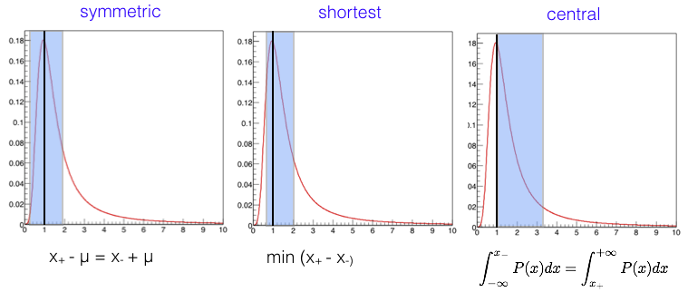
Fig. 39 Example of intervals on an asymmetric p.d.f.

Confidence belt - Neyman/Frequentist construction

The general way to communicate the statistical uncertainty on a measurement is to give a confidence interval. In this section we will describe the frequentist/classical construction given by Neyman in 1937.

Before going to the formal construction let’s take a look at an example to show a common pitfall.

Example:

The weight of an empty dish is measured to be \(25.30 \pm 0.14\) g. A sample of powder is placed on the dish, and the combined weight measured as \(25.50 \pm 0.14\) g. By subtraction and error propagation the weight of the powder is \(0.20 \pm 0.20\) g. This is a perfectly sensible results. However, look at what happens to the probabilities. The naive statement now says that there is a 32% chance of the weight being more than \(1~\sigma\) away from the mean, which is evenly split, making a 16% chance that the weight is negative ! [@Barlow]

The general issue addressed by the construction of the confidence belt is how to turn the knowledge from a measurement \(x\pm \sigma\) into a statement about the value X of the random variable.

Suppose you have a set of measurements \(\{x_1,\ldots,x_n\}\) and you use them to compute the observed value of an estimator \(\hat{\theta}(x_1,\ldots,x_n) = \hat{\theta}_{obs}\). Suppose also that given any “true value” of \(\theta\) you are able to compute the pdf of \(\hat{\theta}\): \(g(\hat{\theta},\theta)\). From the p.d.f. \(g(\hat{\theta},\theta)\) (see Fig. 40) we can determine two values \(u_\alpha\) and \(v_\beta\) such that there is a probability \(\alpha\) to observe \(\hat{\theta} \geq u_\alpha\) and \(\hat{\theta} \leq v_\beta\).

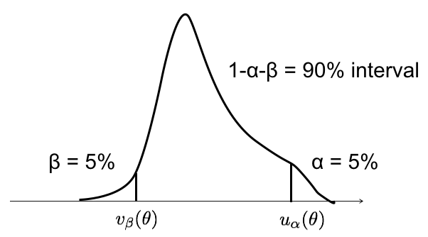
Fig. 40 Example of \(g(\hat{\theta},\theta)\).

The values of \(u_\alpha\), \(v_\beta\) depends on the true value of \(\theta\) and, because we know the p.d.f. \(g(\hat{\theta},\theta)\), we can compute them inverting: $\(\label{eq:alpha} \alpha = P(\hat{\theta} \geq u_\alpha(\theta)) = \int_{u_\alpha(\theta)}^\infty g(\hat{\theta},\theta) d\hat{\theta}\)$

\[\beta = P(\hat{\theta} \leq v_\beta(\theta)) = \int_{-\infty}^{v_\beta(\theta)}g(\hat{\theta},\theta) d\hat{\theta}\]

We can now “build horizontally” as in in Fig. 41.

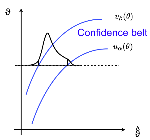
Fig. 41 Example of how to built “horizontally” a confidence belt.

For each value of \(\theta\) on the y-axis you compute the boundaries \(u_\alpha\), \(v_\beta\). By scanning the whole y-axis you obtain two curves \(u_\alpha(\theta)\) and \(v_\beta(\theta)\). The region in between the two curves is called confidence belt. By construction, for any value of \(\theta\) the probability for the estimator to be inside the belt is

\[ P(v_\beta(\theta) \leq \hat{\theta} \leq u_\alpha(\theta)) < 1 -\alpha - \beta. \]

Now we can “read the plot vertically” (see Fig. 42: take your data and compute the observed value \(\hat{\theta}_{obs}\). Now take that value and read off the plot on the y-axis \(a(\hat{\theta})\) and \(b(\hat{\theta})\). The interval \([a,b]\) is the confidence interval at a confidence level \(1-\alpha - \beta\). Note that you’re making a statement about the interval you choose, not on the value of \(\theta\).

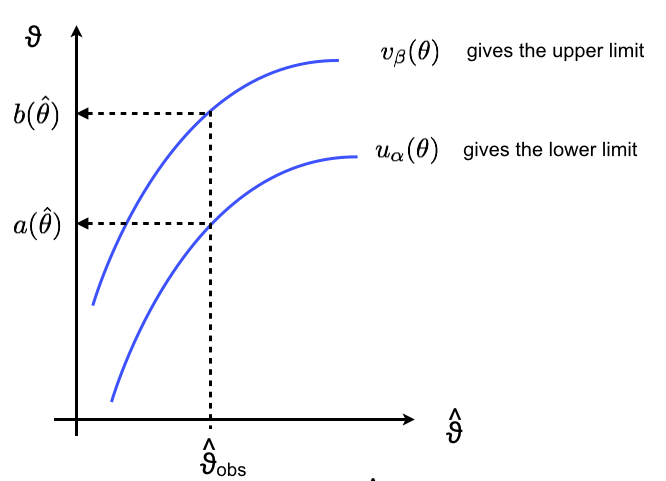
Fig. 42 Example of how to read “vertically” a confidence belt.

Formally you need to require that the two functions \(u_\alpha(\theta)\) and \(v_\beta(\theta)\) are monotonically increasing (which is generally the case for well behaved estimators) and so you can invert them: $\(a(\hat{\theta}) = u^{-1}_\alpha(\hat{\theta}) \qquad ; \qquad b(\hat{\theta}) = v^{-1}_\beta(\hat{\theta})\)$ If that is the case then you can translate the inequalities

(12)\[\hat{\theta} \geq u_\alpha(\theta) \qquad ; \qquad \hat{\theta} \leq v_\beta(\theta)\]

into

(13)\[a(\hat{\theta}) \geq \theta \qquad ; \qquad b(\hat{\theta}) \leq \theta .\]

So the Eq.(12) and Eq.(13) become

\[ P(a(\hat{\theta}) \geq \theta) = \alpha \qquad ; \qquad P(b(\hat{\theta})\leq \theta) = \beta \]

which proves that \(P(a(\hat{\theta}) \leq \theta \leq b(\hat{\theta})) = 1-\alpha-\beta\).

Here and in the following, we will use the convention used by Cowan also keeping the term “significance level” for the goodness of fit and using “confidence level” for the coverage probability of a confidence interval.

The confidence level is also called coverage probability because, from a frequentist point of view, if the experiment were to be repeated many times, the interval \([a,b]\) would cover the true (unknown) value \(\theta_{true}\), \(1-\alpha-\beta\) of the times.

The confidence interval \([a,b]\) is typically expressed by reporting the result of a measurement as \(\hat{\theta}_{-c}^{+d}\) where \(c = \hat{\theta}-a\) and \(d = b-\hat{\theta}\). These values for a central confidence level of 68% are also the one used to represent graphically the error bars.

The case we have just treated is the so called “two-sided” confidence interval. There are however cases where we might be interested in giving only a one sided interval:

• lower limit \(a \leq \theta\) with coverage probability \(1-\alpha\)

• upper limit \(\theta \leq b\) with coverage probability \(1-\beta\)

The value \(a\) is the value of \(\theta\) for which a fraction \(\alpha\) of the measurements would be higher than the observed one (and similarly for \(b\)). To get the value of \(a\) (\(b\)) we have to solve (typically numerically) the equation for a (\(b\)):

\[ \alpha = \int_{\hat{\theta}_{obs}}^\infty g(\hat{\theta},a) d\hat{\theta} \]

\[ \beta = \int_{-\infty}^{\hat{\theta}_{obs}}g(\hat{\theta},b) d\hat{\theta} \]

Example:

Let’s take as an example a gaussian distributed estimator with mean \(\theta\) (true value unknown) and standard deviation \(\sigma_{\hat{\theta}}\) (known; if unknown you can estimate it from data getting \(\hat{\sigma}_\theta\) and move from the gaussian to the Student’s \(t-\)distribution). The gaussian estimator is very common thanks to the central limit theorem (where any estimator that is a sum of random variables is approximately gaussian in the large sample limit). The integrals in Eq.(12) and Eq.(13)   become the well known cumulative functions of the gaussian:

\[ G(\hat{\theta},\theta,\sigma_{\hat{\theta}}) = \int_{-\infty}^{\hat{\theta}} \frac{1}{\sqrt{2 \pi \sigma_{\hat{\theta}}^2}} exp\left( \frac{-(\hat{\theta}' - \theta)^2}{2\sigma_{\hat{\theta}^2}} \right) d\hat{\theta}' \]

and the general case exposed above, simplifies considerably. We need to solve for \(a\) and \(b\) the equations:

\[ \alpha = 1-G(\hat{\theta}_{obs},a,\sigma_{\hat{\theta}}) = 1 - \Phi\left( \frac{\hat{\theta}_{obs} - a}{\sigma_{\hat{\theta}}}\right) \]

\[ \beta = G(\hat{\theta}_{obs},b,\sigma_{\hat{\theta}}) = \Phi\left( \frac{\hat{\theta}_{obs} - b}{\sigma_{\hat{\theta}}}\right) \]

that can be easily done by using the quantile of the gaussian \(\Phi^{-1}\) (the inverse function of \(\Phi\)):

\[ a = \hat{\theta}_{obs} - \sigma_{\hat{\theta}} \Phi^{-1}(1-\alpha) \]

\[ b = \hat{\theta}_{obs} + \sigma_{\hat{\theta}} \Phi^{-1}(1-\beta) \]

where we used \(\Phi^{-1}(\beta) = -\Phi^{-1}(1-\beta)\). Thus, the general curve for \(u_\alpha(\theta)\) and \(v_\beta(\theta)\) become linear function.

Example:

Another very frequent case is when the estimator is a Poisson variable \(n\). Suppose you have performed a measurement and you found \(\hat{\nu}_{obs} = n_{obs}\) and from this you want to build the confidence interval for the mean \(\nu\) (see Fig. 43. The procedure is the same as for the general case shown above, but here we are dealing with a discrete variable. This means that in general, once \(\alpha\) and \(\beta\) are fixed, because \(\hat{\nu}\) can only take discrete values, the Eq.(12), Eq.(13) only holds for particular values of \(\nu\) (and in general because of rounding we will give conservative intervals). Using the Poisson p.d.f. we have these equations to solve numerically:

\[ \alpha = \sum_{n=n_{obs}}^\infty f(n;a) = 1 - \sum_{n=0}^{n_{obs}-1}f(n;a) = 1 - \sum_{n=0}^{n_{obs}-1}\frac{a^n}{n!}e^{-a} \]

\[ \beta = \sum_{n=0}^{n=n_{obs}}f(n;b) = \sum_{n=0}^{n_{obs}} \frac{b^n}{n!}e^{-b} \]

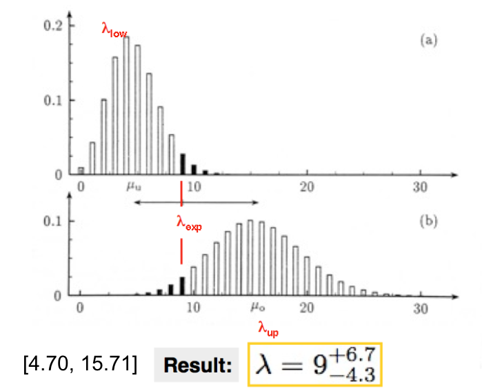
Fig. 43 Here we observed 9 radioactive decays and we constructed the 90% symmetric CL \(\lambda \in [\lambda_{low}-9, \lambda_{up}-9]\), i.e. \(\lambda = 9^{+6.7}_{-4.3}.\)

Upper limit when \(n_{obs} = 0\): Again from the formulas in the previous example, you can compute what is the upper limit on the frequency of a rare event in case you don’t observe any. At \(1-\beta = 95\)% CL you get \(b=2.996\), typically rounded to 3. This is why anytime you see a paper with zero observed events the quoted upper limit is 3.

Error bars on empty bins: From the formulas in the example above we can see that the upper limit \(b\) when \(n_{obs} = 0\) becomes \(\beta=e^{-b}\). If we set the central confidence level at \(1-\beta=0.6827\) we find \(b=-\log(0.3173/2) \sim 1.8\). This is the reason of the error bar at 1.8 when we observe zero events in a counting experiment. (In FIXME ROOT you can get the correct Poisson error bars using the method TH1::SetBinErrorOption(TH1::kPoisson)).

When the p.d.f. of the estimator is not a gaussian, and approximating it to a gaussian would lead to biases or under/over coverage of the confidence interval, one can always extract the p.d.f. of the estimator tossing toy experiments and compute the confidence belt numerically. In some specific cases one can also try to transform the estimator such that the transformed variable is gaussian distributed.

Example:

Consider, as an example for which the p.d.f. of the estimator is not gaussian, the correlation coefficient \(\rho\) of a two-dimensional gaussian and the estimator \(r\) as

\[ r=\frac{\sum_{i=1}^n(x_i-\bar{x})(y_i-\bar{y})}{\left( \sum_{j=1}^n(x_j-\bar{x})^2\cdot\sum_{k=1}^{n}(y_k-\bar{y}) \right)^{1/2}} \]

The distribution for this estimator is shown in Fig. 44 and it only approaches a gaussian distribution in the large sample limit.

For this specific case, Fisher showed that the transformed estimator

\[ z=\tanh^{-1} r = \frac{1}{2} \log\frac{1+r}{1-r} \]

reaches the gaussian limit much more quickly. You can use this transformation for an estimator \(\zeta\)

\[ \zeta = \tanh^{-1} \rho = \frac{1}{2} \log\frac{1+\rho}{1-\rho} \]

The expectation value and the variance for \(z\) are approximately given by:

\[ <z> = \frac{1}{2}\log\frac{1+\rho}{1-\rho} + \frac{\rho}{2(n-1)} \qquad ; \qquad V[z] = \frac{1}{n-3} \]

Assuming that the sample is large enough such that you can neglect the bias \(\frac{\rho}{2(n-1)}\), you can use these to determine the confidence interval \([a,b] = [z-\hat{\sigma}_z,z+\hat{\sigma}_z]\) such that the lower limit \(a\) for \(\zeta\) is at confidence level \(1-\alpha\) and the upper limit \(b\) is at \(1-\beta\) confidence level. From \([a,b]\) on \(\zeta\) you can go back to the interval \([A,B]\) on \(\rho\) simply inverting \(\zeta = \tanh^{-1} \rho\) (\([A = \tanh \alpha, B = \tanh\beta]\)).

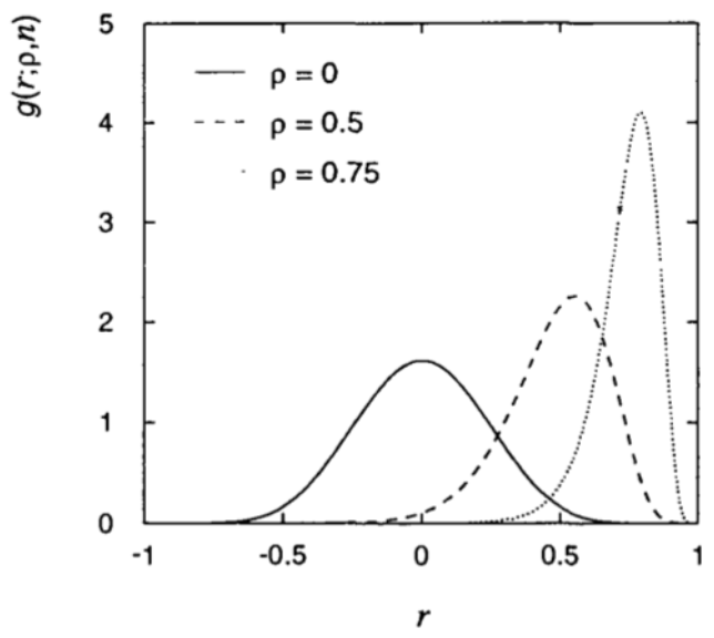
Fig. 44 Distribution of the correlation estimator for a sample of size n=20 and different values of \(\rho\).

Use the likelihood or the \(\chi^2\) to set confidence intervals

In the large sample limit approximation it is easy to extract confidence intervals using the likelihood method or equivalently the \(\chi^2\) method (\(L=\exp(-\chi^2/2)\)).

In the gaussian case, as we have already seen when estimating the uncertainty on the likelihood estimator, we can get the estimated \(\hat{\sigma}_{\hat{\theta}}\) for \(\sigma_{\hat{\theta}}\) from:

\[ \log ~L(\hat{\theta} \pm N \sigma_{\hat{\theta}}) = \log L_{max} - \frac{N^2}{2} \]

and again as we have already seen, this amounts to move by 0.5 from the maximum value. Even if the likelihood is not gaussian the central confidence interval \([a,b] = [\hat{\theta}-c, \hat{\theta}+d]\) can still be approximated by:

\[ {\color{blue}{LIKELIHOOD}}~:~\log ~L(\hat{\theta}^{+d}_{-c}) = \log L_{max} - \frac{N^2}{2} \qquad \; \qquad {\color{blue}{\chi^2}}~:~\chi^2(\hat{\theta}^{+d}_{-c}) = \chi^2_{min} + N^2 \]

for the likelihood and the \(\chi^2\) methods respectively, where \(N=\Phi^{-1}(1-\gamma/2)\) is the quantile of the standard gaussian distribution corresponding to the desired confidence level. The \(\chi^2\) prescription is just the likelihood one where we use \(\log L=-\chi^2/2\). This is by far the most used method to report the statistical uncertainties, but it has to be remembered that it exact only for gaussian likelihood or in the large sample limit and for all other cases it is only an approximation !

Example:

Consider the lifetime measurement of an unstable particle. We can extract the value of the lifetime by fitting the exponential distribution of the proper decay time of a large number of particles.

The ML estimator comes out to be just the average \(\hat{\tau}=\frac{1}{n}\sum_{i=1}^{n}t_i\). For a small statistics as in Fig. 45, where we only have 5 measurements, the likelihood is non parabolic and it is preferable to report the asymmetric values given by \(\log L_{max} - \frac{1}{2}\): i.e. \([\hat{\tau} - \Delta\hat{\tau}_-, \hat{\tau} + \Delta\hat{\tau}_+]\).

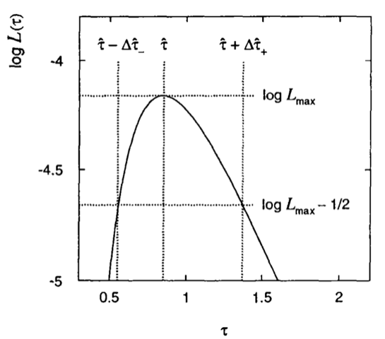
Fig. 45 Non-parabolic log-Likelihood scan of a lifetime measurement done on a small statistics sample.

The same method can be applied to find confidence intervals in several dimensions (a.k.a. confidence regions). What in one dimension was an interval in n-dimensions becomes a region bounded by an hyper-ellipsoid defined by constant values of \(Q(\vec{\hat{\theta}},\vec{\theta})\).

If \(\vec{\hat{\theta}}\) is described by a n-dimensional gausssian p.d.f. \(g(\vec{\hat{\theta}}, \vec{\theta})\) ,then \(Q(\vec{\hat{\theta}}, \vec{\theta})\) is distributed according to a \(\chi^2\) distribution with n degrees of freedom. We can then compute the probability to have the estimate \(\vec{\hat{\theta}}\) near the true value (and viceversa) as

\[ P(Q(\vec{\theta},\vec{\hat{\theta}}) < Q_\gamma) = \int_0^{Q_\gamma} f(z;n)dz = 1-\gamma \]

where \(f(z;n)\) is the \(\chi^2\) distribution with n degrees of freedom. Inverting using the quantile of the \(\chi^2\) distribution we get:

\[ Q_\gamma = F^{-1}(1-\gamma;n) \]

The region defined by the \(Q(\vec{\theta},\vec{\hat{\theta}}) < Q_\gamma\) is called confidence region with confidence level \(1-\gamma\). In the case of a gaussian likelihood, the confidence region can be constructed by finding the region of the space such that:

\[ \log L(\vec{\theta}) = \log L_{max} - \frac{Q_\gamma}{2} \]

Typical values of the quantiles of the \(\chi^2\) distribution are listed in Fig. 46. Note that for increasing number of dimensions the confidence level, at a fixed quantile \(Q_\gamma\) decreases.

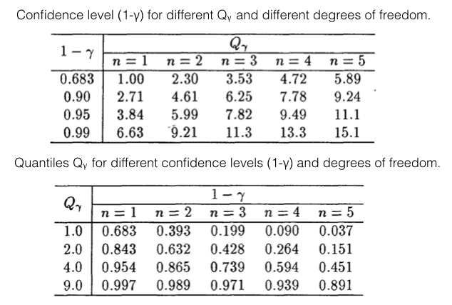
Fig. 46 Quantiles and confidence levels in n-Dimensions.

Limits near boundaries

When performing searches, very often we are faced with the problem of looking for a new effect at the boundaries of the phase space. Suppose we want to measure the neutrino mass; because of the oscillation phenomenon we know neutrinos are not (all of them) massless. Still their mass is very small, i.e. near the boundary m = 0.

Deciding how to quote the result of a measurement after seeing the results is called “flip-flop” and will be addressed using the Feldman-Cousins construction in Sec. Flip-Flop.

Depending on the resolution of the measurement, we typically face two situations:

• the data yields a value significantly different from zero; we will then quote the measured value with an uncertainty

• the data yields a value compatible with zero; we will then proceed to quote an upper limit on the value of the parameter at a given CL.

The problem gets trickier when the estimator takes values in a physically forbiddend region. To get the idea: suppose you measure a mass as \(m^2 = E^2 - p^2\). Depending on the uncertainties on energy and momentum you can obtain negative values for the mass. From the purely statistical point of view you can proceed as before and set the upper limit \(\theta_{up}\) at \(1-\beta\) CL is given by:

\[ \theta_{up} = \hat{\theta}_{obs} + \sigma_{\hat{\theta}}\Phi^{-1} (1-\beta). \]

The interval \((-\infty, \theta_{up})\) will contain the true value of \(\theta\) with a probability of 95%.

Now, take as an example a measurement giving \(\theta_{obs} = -2.0\) with a standard deviation \(\hat{\sigma}=1\): the upper limit is \(\theta_{up} = -0.355\) at 95% CL. We are setting a negative upper limit on a mass! Having a negative upper limit has to happen 5% of the times when using a 95%CL. We just got one of the 5%. The annoying point is that, because we knew from the beginning that the mass has to be positive, the experiment does not bring any new piece of information. In such a case we should still quote the value we found such that, when combined with more experiments, we will contribute to the measurement of the correct value. If you encounter a very asymmetric likelihood, you should in general publish the scan of the likelihood on the parameter you are estimating.

A naive approach to avoid the negative upper limit is to shift the negative estimate to the boundary (\(\hat{\theta}=0\) in this case):

\[ \theta_{up}=max(\hat{\theta}_{obs},0) + \sigma_{\hat{\theta}}\Phi^{-1} (1-\beta). \]

In this case, if the limit is positive you will quote the same value given by the classical construction, while for negative values you will end up with an unwanted coverage larger than the quoted \(1-\beta\).

The most natural way to include boundaries in the computation of limits is to use the Bayes theorem:

\[ p(\theta|x) = \frac{L(x|\theta)\pi(\theta)}{\int L(x|\theta')\pi(\theta')d\theta'} \]

where \(L(x|\theta)\) is the likelihood to observe a value \(x\) given the parameter \(\theta\) and \(\pi(\theta)\) is the prior on \(\theta\). The most probable value of the posterior \(p(\theta|x)\) coincides with the ML estimator if the prior is flat (the denominator only contributes as a normalization constant). To set limits (without considering boundaries for the moment), we can use the expression for the posterior and find numerically the interval \([a,b]\) such that:

\[ \alpha = \int_{-\infty}^{a}p(\theta|x)d\theta \qquad \beta =\int_{b}^{+\infty}p(\theta|x)d\theta \]

where \(\alpha\) and \(\beta\) define the CL.

Using the Bayes theorem, the inclusion of boundaries is trivial: we just need to write them in the prior. In the example of a mass limited to positive values, we can write the prior to be zero for negative masses and flat above:

\[\begin{split} \pi(\theta) = \left\{ \begin{array}{rll} 0 & \mbox{if} & \theta \le 0 \\ 1 & \mbox{if} & \theta > 0 \end{array}\right. \end{split}\]

The upper limit on the mass will be found as before by solving numerically for \(\theta_{up}\) the integral on the posterior:

\[ 1-\beta = \int_{-\infty}^{\theta_{up}} p(\theta|x) = \frac{\int_{-\infty}^{\theta_{up}}L(x|\theta)\pi(\theta)d\theta }{\int_{-\infty}^{+\infty}L(x|\theta)\pi(\theta)d\theta }{} \]

This method is clearly affected by the issues on the encoding of ignorance in the prior (i.e. the choice of a flat prior):

• using a flat prior assumes that the probability for the parameter \(\theta\) is the same everywhere in the physically allowed phase space; applied to the neutrino mass example, this would mean that the probability is the same in the range \([0,1]\)eV as in \([10^{10}, 10^{10}+1]\)eV.

• a flat prior won’t remain flat under a non-trivial transformation of the parameter \(\theta\).

With the Bayes approach, you don’t need anymore to go for the “build horizontally / read vertically” classical construction. You just need to compute the integrals above. For the example of the neutrino mass: the denominator is an integral on the full phase space \((0,+\infty)\), while the numerator runs on \((0, \theta_{up})\). For large values of \(x = \theta_{obs}\) the bayesian limit approaches the classical one: the likelihood you are integrating is far from the boundary and the tail below zero is negligible. The closer you get to the boundary the larger is the area of the likelihood leaking in the unphysical region. Still, the upper limit will never cross zero because it is extracted from the ratio of two integrals where the numerator is by construction always a fraction of the denominator.

Fig. 47 shows the comparison of the different methods discussed so far: the classical construction; the “shifted” classical construction where the upper limit if forced to be flat for \(\hat{\theta}<0\); and the bayesian approach where the upper limit on \(\theta\) never falls below zero.

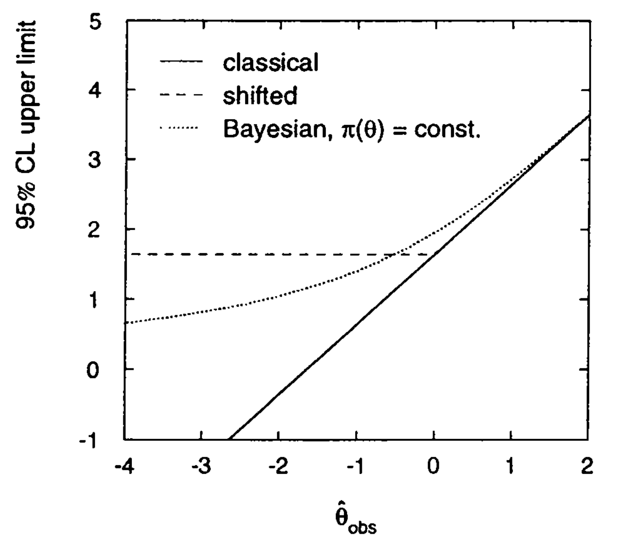
Fig. 47 Comparison of the upper limits obtained with the classical construction, the “shifted” classical construction and the bayesian approach.

Another frequent case is when we try to set an upper limit on a rare signal with a counting experiment. Here the boundary is given by the number of events that has to be greater or equal than zero. Let’s start from the simpler situation where we don’t set any constraint (or equivalently we are far away from the boundary) and compute the upper limit following the classical construction. We observe \(n\) events some of which come from signal \(n_s\) and some others from background \(n_b\): \(n = n_s+n_b\). The number of events follow a Poisson distribution with an expected number of events \(\nu_s\) for signal and \(\nu_b\) for background (suppose we know the expected number of background events with negligible uncertainty). We want to get the upper limit on the number of signal events in the sample. The ML estimator for the number of signal events is simply \(\hat{\nu}_s = n - \nu_b\). The confidence interval can be extracted as usual by solving (numerically) the equation:

\[ \beta = P(\hat{\nu}_s\leq\hat{\nu}_s^{obs}| \nu^{up}) = \sum_{n\leq \hat{\nu}_{obs}}\frac{(\nu_s^{up} + \nu_b)^n e^{(\nu_s^{up} + \nu_b)}}{n!} \]

The results for some values of observed events and expected backgrounds are shown in Fig. 48.

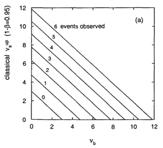
Fig. 48 Upper limit on the number of signal events as a function of the expected number of background events \(\nu_b\) for different observed \(n\).

Before moving to the Bayesian solution to setting the upper limit, let’s see where the classical one ends into troubles. Suppose you have a small number of expected signal events and large background. In this situation the number of observed events will be dominated by the background and we can find cases where the number of observed events is smaller than the expected number of background events (e.g. \(\nu_b\) = 8, \(n\) = 1). By reading off the limit from Fig. 48 we find a negative number of signal events. As we have already seen for the example of the neutrino mass measurement this is not wrong. We are setting an upper limit at 95% CL and we got one large downward fluctuations which should happen in 5% of the cases. Nevertheless from a physics content the result is not particularly interesting (we knew before setting up the experiment that the number of events has to be greater than or equal to zero).

Using the bayesian approach the posterior can be written as:

\[ p(\nu_s|n_{obs}) = \frac{L(n_{obs}|\nu_s)\pi(\nu_s)}{\int L(n_{obs}|\nu_s')\pi(\nu_s')d\nu_s'} \]

To include the boundary \(\nu_s>0\) we can simply define the prior as:

\[\begin{split} \pi(\nu_s) = \left\{ \begin{array}{rll} 0 & \mbox{if} & \nu_s \le 0 \\ 1 & \mbox{if} & \nu_s > 0 \end{array}\right. \end{split}\]

To compute the upper limit we just need to plug this prior in the posterior expression $\( 1-\beta = \frac{\int_{0}^{\nu_s^{up}}L(n_{obs}|\nu_s)d\nu_s }{\int_{0}^{+\infty}L(n_{obs}|\nu_s)d\nu_s} \)$

and solve numerically for \(\nu_s^{up}\). The equivalent of Fig. 48 using a bayesian approach is shown in Fig. 49.

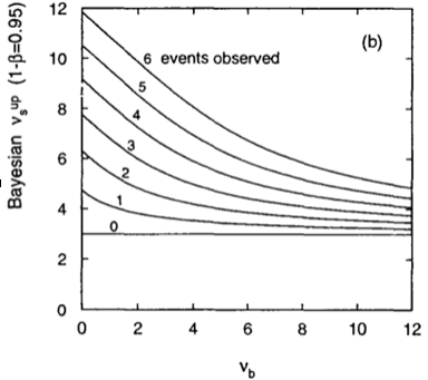
Fig. 49 Bayesian upper limit on the number of signal events as a function of the expected number of background events \(\nu_b\) for different observed \(n\).

The bayesian limit is always greater or equal than the classical one. As expected the bayesian approaches the classical limit when we move to the region where the number of observed events is much larger than the number of expected background events. The fact that the two limits precisely coincide for \(n_{bkg}=0\) is a pure coincidence since the Bayesian limit depends on the particular choice of the prior.

Feldman-Cousins

The Feldman-Cousins (FC) prescription of the confidence intervals solves two complications related to the classical Neyman construction: the so called “flip-flop” problem and the problem of obtaining unphysical (or empty set) interval using the Neyman construction. Their solution provides, in a purely frequentist manner, intervals which are never unphysical, nor empty and unifies the set of classical confidence intervals for setting upper limits and quoting two-sided confidence intervals. However, it still suffers from an apparent paradox when the number of observed events is lower than the background only expectations (background underfluctuations).

*In this section we will follow closely the paper in Ref. [FC98].

The flip-flop problem

The flip-flop problem arises when one decides, based on the results of the experiment, whether to publish an upper limit or a central confidence interval. This is a very common (and sensible) attitude. Typically the reasoning goes as: if I see that a result is below 3\(\sigma\) I publish an upper limit, if the result has a significance of more than 3\(\sigma\) then I publish a central confidence interval. The typical sentence in papers is: “the data are compatible with the background expectations (or no excess is observed above the expected background) hence we set an upper limit on…”. As seen in the previous section, one can even decide that in case of a boundary, e.g. a mass which has to be positive, to use the maximum between the measured value and zero \(\max(m,0)\) and quote the CL corresponding to zero. These choices has an impact on the coverage of the reported confidence intervals.

To better understand the flip-flop problem we start by looking at the confidence belt at 90% CL of Fig. 50(left). Here we are considering a gaussian observable with \(\sigma=1\); the \(x\)-axis is the measured mean \(x\), while the \(y\)-axis is the unknown mean \(\mu\). By construction the coverage is 90%, i.e. reading the plot vertically for a measured \(x\), we have \(P(\mu \in [\mu_1,\mu_2]) =90\%\). The corresponding plot for the upper limit at 90%, again using the classical construction, is shown in the Fig. 50(right).

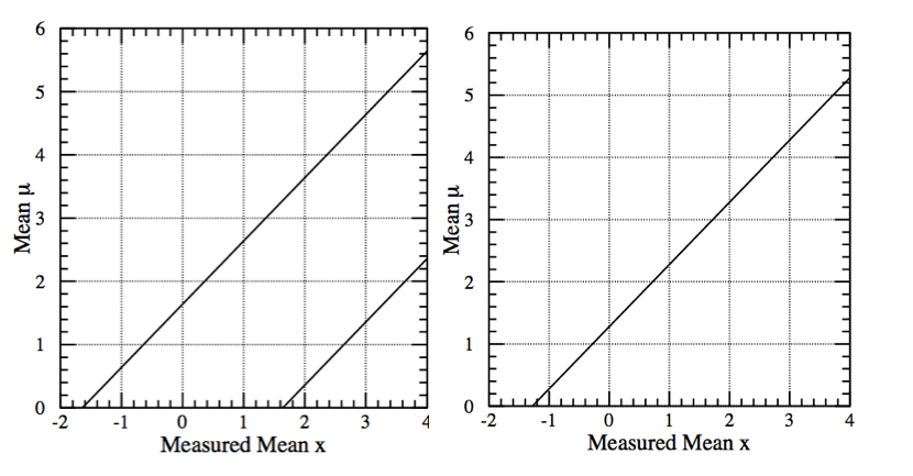
Fig. 50 (left) 90% CL confidence belt; (right) 90% CM upper limit.

If you decide decide a posteriori (i.e. based on the result of the measurement) whether to publish a central confidence interval, an upper limit or the truncated \(\max(x,0)\) limit, you will get a confidence region such as the one reported in Fig. 51.

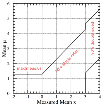
Fig. 51 “A posteriori” confidence interval: if the result x is more than \(3\sigma\) (i.e. x \(>\) 3) publish the central confidence interval; if the result x is less than \(3\sigma\) (i.e. x \(<\) 3) publish an upper limit; if the results is negative use max(meas,0) and quote the CL corresponding to 0.

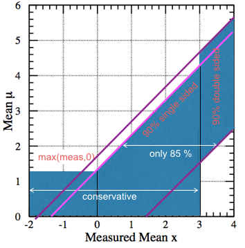
Fig. 52 The interval doesn’t have the correct coverage.

This region does not guarantee the 90% coverage. It’s not “built horizontally” following the classical construction; it’s a patchwork of confidence intervals. Take for example the case of \(\mu=2\) (see Fig. 52. The interval starts with the lower limit at \(2-1.28\) on the boundary of the 90% upper limit and ends at \(2+1.64\) on the \(90\%\) central interval, giving a coverage of only \(1-0.1-0.05 = 85\%\). In other cases, like at \(\mu=1\) the region over-covers as shown in the same figure, the confidence region overcovers. We will see in the following how the FC prescription allows to unify these intervals and avoid the problem.

Typically the flip-flop problem only comes if you publish a confidence interval for a well established signal, but with more data the signal disappears and you are forced to set a limit. While potentially this could be a very serious issue, in reality it only happens very rarely because the experimental sensitivity typically grows with additional data.

Poisson with background

To understand the FC prescription we will use the example of a counting experiment. The measured number of events is \(n\), the number of expected background events is \(b\) (set to \(b=3\) in this example) and we want to build the confidence interval for the mean \(\mu\):

\[ P(n|\mu) = \frac{(\mu+b)^n}{n!}e^{-(\mu+b)} \]

Let’s start from the classical construction of the upper limit (UL) as seen in

Sec.Confidence Intervals (see Fig. 53).

We build horizontally the UL curve scanning the \(y\)-axis (the unknown signal mean) \(\mu\) and for each value of \(\mu\) we find the value of the limit solving numerically for \(\mu\) the equation \(0.1=\sum_0^{n_{obs-1}}P(n|\mu+b)\). See Fig. 43 for a graphical reminder of the procedure. Following the same procedure we can built the confidence interval for the central interval at \(CL=90\%\). In this case the lower and upper limits are computed solving numerically for \(c\) in \(0.05=\sum_0^{n_{obs-1}}P(n|c+b)\) and for \(a\) in \(0.05=\sum_{n_{obs}}^\infty P(n|a+b)\). When \(n=0\) we get an empty set. For both the upper and central limits, n = 0 has no solution (in the example b = 3). This is counter-intuitive: if one measures no events, clearly the most likely value of \(\mu\) is zero. Why should one rule out the most likely scenario? Let’s see how this issue is addressed using the FC prescription.

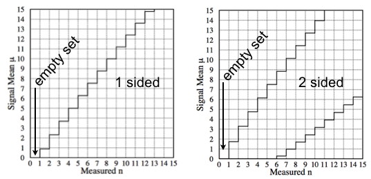
Fig. 53 90% CL upper limit (left) and confidence interval (right) following the classical construction. for the case with expected background \(b=3\).

The FC uses the classical Neyman construction, but using a different ordering principle. Every time a confidence region is defined, we use (often without even noticing) the concept of ordering principle. An ordering principle is needed to specify which values of the measured \(x\) to include in the acceptance region. When building an upper limit we start from the smallest values of \(x\), for a central limit we start from the value of \(x\) closest to the central value, etc… There are infinite ordering principles. The FC ordering uses an ordering principle based on a likelihood ratio.

To understand the idea let’s take the example where we want to build horizontally the interval for \(\mu=0.5\) (remember we set the number of background events \(b=3\)). The Poisson probability to obtain \(0\) events, when the expected number of events is \(\mu = 0.5\) is 0.03. Let’s compare this low value with the one we obtain using as \(\mu\) the most probable \(\mu_{best}\). \(\mu_{best}\) is defined as the value of the mean signal \(\mu\) which maximizes \(P(n|\mu)\) when we require \(\mu_{best}\) to be physically allowed (i.e. \(\mu_{best}>0\)). This simply means (remembering the ML estimator for a signal in presence of background) \(\mu_{best} = max(0,n-b)\). The probability to obtain \(0\) events when the expected number of events is \(\mu_{best} = 0\) is 0.05. So, while \(P(n,\mu=0.05)=0.03\) is quite low on an absolute scale, it is very much comparable with \(P(n,\mu_{best}=0)=0.05\) of the most probable value \(\mu_{best}\).

Following this observation the ordering principle is defined on the likelihood ratio:

\[ R(\mu) = \frac{P(n|\mu)}{P(n|\mu_{best})} \]

where \(R\) is called rank. The effect of this ordering principle is to increase the rank of the values with low probability if they are close to \(\mu_{best}\). The interval is then built by including values of \(n\) in decreasing order of \(R\) until the sum of \(P(n|\mu)=1-CL\) i.e. matches the CL we want. Due to the discreteness of \(n\), the acceptance region can contain more summed probability than required by the CL, i.e. we could end up over-covering. Notice that while in the typical orderings different values of \(\mu\) do not talk to each other, here \(\mu_{best}\) influence the “weight” of all the other values (their order).

Let’s compute the interval for the numerical example used above (expected number of background events is \(b=3\), we measure \(n\) events and we want to build the confidence interval for \(\mu=0.5\)).

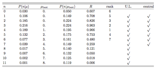
Fig. 54 Confidence interval construction for \(\mu=0.5\) and background \(b=3\).

For each value of \(n\) we first compute \(\mu_{best}\) the best (physical) value of the estimator given n (see table in Fig. 54. We get \(\mu_{best} = max(0,n-b)\): \(n=0 \to \mu_{best}=0\), \(n=1 \to \mu_{best}=0\), \(n=2 \to \mu_{best}=0\), \(n=3 \to \mu_{best}=0\), \(n=4 \to \mu_{best}=1\), \(n=5 \to \mu_{best}=2\),…. For each \(n\) we also compute \(P(n|\mu=0.05)\) and \(P(n|\mu_{best})\) and the rank \(R=P(n|\mu=0.05)/P(n|\mu_{best})\). Now we can complete the confidence interval. We add the probabilities \(P(n|\mu=0.05)\) in decreasing order of the rank \(R\) until we match the desired CL:

\[\begin{split} \begin{aligned} P(4|\mu=0.05) & + P(3|\mu=0.05) + P(2|\mu=0.05) + P(5|\mu=0.05) + P(1|\mu=0.05) + \\ & P(0|\mu=0.05) + P(6|\mu=0.05) = \\ 0.189 & + 0.216 + 0.185 + 0.132 + 0.106 + 0.030 + 0.077 = 0.935 \end{aligned} \end{split}\]

We intentionally stay on the conservative side and add passed 0.9. The alternative would be to stop at \(R=6\) which is \(0.858 < 0.9\), hence under-covering. Repeating the procedure scanning the values of \(\mu\) on the \(y\)-axis we obtain the complete confidence belt.

The resulting FC confidence interval is compared with the classical one in Fig. 55.

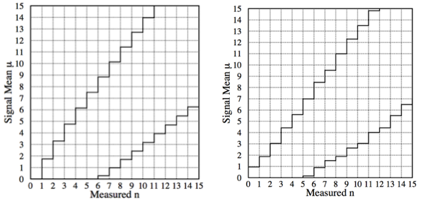
Fig. 55 Comparison of the FC confidence interval with the classical one.

At large \(n\) the FC and the classical construction gives approximately the same confidence interval: we are far away from the physical boundary and so the background is effectively subtracted without constraint. For small values of \(n\) , the confidence interval automatically becomes upper limits on \(\mu\); i.e. the lower endpoint is 0 for \(n \leq 4\) in this case. Thus, flip-flopping between the plots in Fig. 53 is replaced by one coherent set of confidence interval, (and no interval is the empty set).

Gaussian with boundary at the origin

As another example we can build the FC confidence interval for a gaussian distribution with a boundary \(\mu>0\) (e.g. the physical boundary imposed on the mass being positive). and compare it with what we have already encountered in the example in Sec.Classical contruction

Consider as p.d.f. a gaussian with \(\sigma =1\):

\[ P(x|\mu) = \frac{1}{\sqrt{2\pi}}e^{-\frac{(x-\mu)^2}{2}} \]

As we did with the Poisson variable we find \(\mu_{best}\) as the value that maximizes \(P(x|\mu)\) and force it to be positive, i.e. we take \(\max(0,\mu_{best})\). The expression for \(P(x|\mu_{best})\) becomes:

\[\begin{split} P(x|\mu_{best}) = \left\{ \begin{array}{rll} 1/\sqrt{2\pi} & \mbox{if} & x \geq 0 \\ \exp(-x^2/2)/\sqrt{2\pi} & \mbox{if} & x<0 \end{array}\right. \end{split}\]

if \(x>0\) then \(\mu_{best} = x\), while if \(x<0\) we have \(\mu_{best} = 0\) (see Fig. 56).

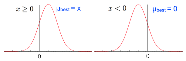
Fig. 56 \(\mu_{best}\) is the value that maximizes \(P(x|\mu)\).

The likelihood ratio is then:

\[\begin{split} R(x) = \frac{P(x|\mu)}{P(x|\mu_{best})} = \left\{ \begin{array}{rll} \exp(-(x-\mu)^2/2) & \mbox{if} & x \geq 0 \\ \exp(x\mu-\mu^2/2) & \mbox{if} & x<0 \end{array}\right. \end{split}\]

With this we can now add to the acceptance region values of x ordering them by their rank. If \(x\) is far from the boundary, the rank is just \(P(x|\mu)\) and we get to the usual ordering. If instead it is close to the boundary the rank develops a tail to the left as shown in Fig. 57 that will modify the ordering.

Fig. 57 The rank is asymmetric.

For a given value of \(\mu\), one finds the interval \([x_1,x_2]\) such that \(\int_{x_1}^{x_2} P(x|\mu)dx = \alpha\) and \(R(x_1) = R(x_2)\) (see Fig. 58 and Fig. 59). The condition that the rank at the two extremes coincides guarantees that the order we used to pick the values of \(x\) is correct. If the rank was higher (or lower) at one extreme, it would mean that those values of \(x\) should have (have not) be used for the interval.

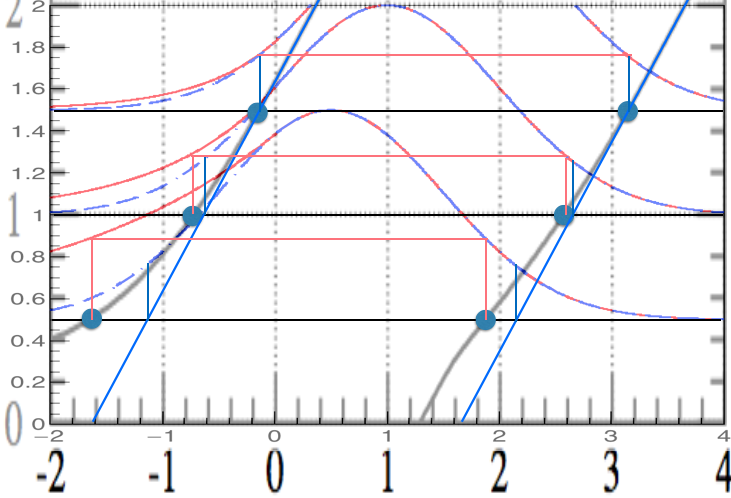
Fig. 58 Classical construction in blue, FC in red.

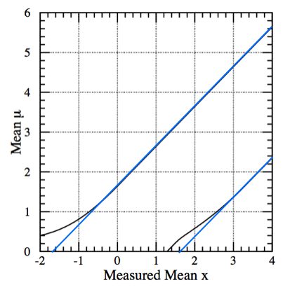
Fig. 59 Classical construction in blue, FC in black.

As expected, far away from the boundary the two intervals coincide. Below \(x=1.28\), the lower endpoint of the FC confidence intervals is zero, so that there is automatically a transition from two-sided confidence intervals to an upper confidence limit given by \(\mu_2\). The point of this transition is fixed by the calculation of the acceptance interval for \(\mu=0\) the solution has \(x_1 =-\infty\), and so \(\int_{x_1}^{x_2} P(x|\mu)dx = \alpha\) is satisfied by \(x_2 =1.28\) when \(\alpha=90\)%.

Neutrino oscillations

The study of neutrino oscillations was the initial reason to develop this methodology. The physics needed to follow the argument is rather simple. Neutrino oscillations originate from the difference between neutrino mass and flavor eigenstates. Considering only two flavors \(\nu_e, \mu_\mu\) we can write the flavor eigenstates as a linear combination of the mass eigenstates:

\[\begin{split} \begin{aligned} |\nu_e \rangle &=& |\nu_1\rangle \cos \theta + |\nu_2\rangle \sin \theta \\ |\nu_\mu\rangle &=& - |\nu_1\rangle \sin \theta + |\nu_1\rangle \cos \theta \end{aligned} \end{split}\]

Studying this two-states quantum mechanical system we obtain that the probability of a \(\nu_\mu\) to oscillate to \(\nu_e\) is :

\[ P(\nu_\mu \to \nu_e) = \sin^2(2\theta)\sin^2\left(\frac{1.27 \Delta m^2 L}{E}\right) \]

where \(\Delta m = |m_1^2 - m_2^2|\) in \(eV^2\), L is the distance in km between the creation and the detection points and E is the energy of the neutrino in MeV. The experimental data are used to measure the oscillations parameters \(\Delta m^2\) and \(\sin^2 2\theta\). The results are usually presented in a 2D plane \((\Delta m^2,\sin^2 2\theta)\) where the excluded values (rejection region) of the parameters are on the right of the boundary (see Fig. 60).

Ignoring the physics behind, just think of this problem as a fit of the data (number of events) to a function of two variables \(f(x,y) = P(\Delta m^2, \sin^2 2\theta)\).

The computation of the excluded region has the complications seen above: the parameter \(\sin^2 2\theta\) is bounded in \([0,1]\) and the expected number of oscillation events is extremely small on a potentially large background.

The neutrino data and the expected background are collected in histograms in bins of energy as \(N=\{n_i\}\) and \(B=\{b_i\}\) respectively. The signal contribution (i.e. the expected number of events coming from oscillations) is collected as a histogram in bins of energy \(T=\{\mu_i|\sin^2(2\theta), \Delta m^2\}\).

To find the upper limits on the oscillation parameters we can use the FC construction. To build the exclusion region (this time is in 2D!) we fix a point in the \((\Delta m^2,\sin^2 2\theta)\) plane (typically the plane is finely binned and instead of a point we approximate one region in the plane with the averaged values of the parameters in that region) and compute the rank of the measured values using as ordering principle the likelihood ratio:

\[ R = \frac{P(N|T(\sin^2(2\theta), \Delta m^2))}{P(N|T(\sin^2(2\theta_{best}), \Delta m_{best}^2))} \]

where \(\sin^2(2\theta_{best}), \Delta m_{best}^2\) are the values giving the highest probability \(P(N|T)\) in the physically allowed range of the parameters. This is equivalent to compute for each bin in the 2D plane:

\[ R = \Delta \chi^2 = 2\sum_i \left( \mu_i -\mu_{best} + n_i\ln\left(\frac{\mu_{best} + b_i}{\mu_i + b_i}\right) \right) \]

Fig. 60 shows the exclusion region on the 2D plane obtained with a toy study. Neutrinos are created uniformly at a distance between 600m and 1000m from the detector with a flat energy spectrum between 10 and 60 GeV. The background flux from \(\nu_\mu\) misidentified as \(\mu_e\) is set to 500 events flat in the energy range. The total \(\nu_\mu\) flux is such that we get 100 events for an oscillation probability \(P(\nu_\mu\to\nu_e)=0.01\). For each toy experiment we compute \(\Delta\chi^2\). For each bin in the \((\Delta m^2,\sin^2 2\theta)\) plane the we need to find \(\Delta \chi^2_c\) such that \(\alpha\) (1-CL) of the simulated experiments have \(\Delta\chi^2 < \Delta\chi^2_c\). To get the exclusion limit from data (the histogram \(N\)) we compute the \(\Delta \chi^2\) for each bin of the \((\Delta m^2,\sin^2 2\theta)\) plane and compare it with the \(\Delta \chi_c^2\) found above. The boundary is given by:

\[ \Delta \chi^2 (N|\sin^2(2\theta),\Delta m^2) < \Delta \chi^2_c(\sin2(2\theta),\Delta m^22). \]

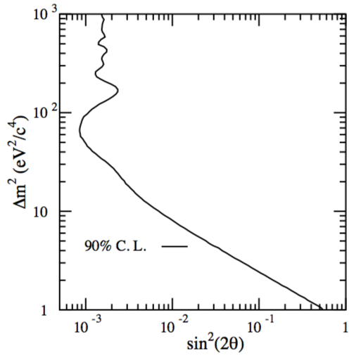
Fig. 60 Confidence region for an example of the toy model in which \(\sin^2(2\theta) = 0\). The 90% confidence region is the area to the right of the curve. In other words the null hypothesis H\(_0\) is no oscillations and with the data at hand I can exclude at 90% CL the region of parameters to the right of the curve.

Other examples

The Feldman-Cousins construction was used in CMS [@Hig12045] for the determination of the intervals on the Higgs measured signal strength (\(\hat{\mu} = \sigma/\sigma_M\) ratio of the measured cross section to the Standard Model expectation). In Fig. 61 the intervals obtained without limiting \(\hat{\mu}\) to be positive and the one imposing \(\hat{\mu}>0\) obtained with the FC prescription. In Fig. 62 the signal strength is fitted on the plane of the different production mechanisms gluon-gluon-fusion-plus-ttH and VBF-plus-VH.

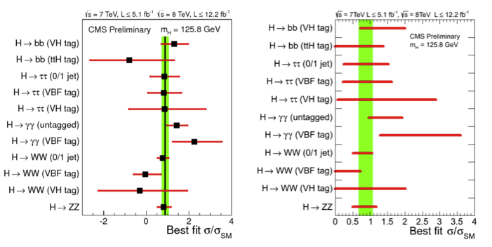
Fig. 61 (left) Values of \(\hat{\mu} = \sigma/\sigma_M\) for the combination (solid vertical line) and for contributing channels (points). The horizontal bars indicate the \(\pm1\sigma\) uncertainties on the \(\hat{\mu}\) values for individual channels; they include both statistical and systematic uncertainties. (right) The same intervals imposing the signal strength to be positive and computed using the Feldman-Cousins construction.

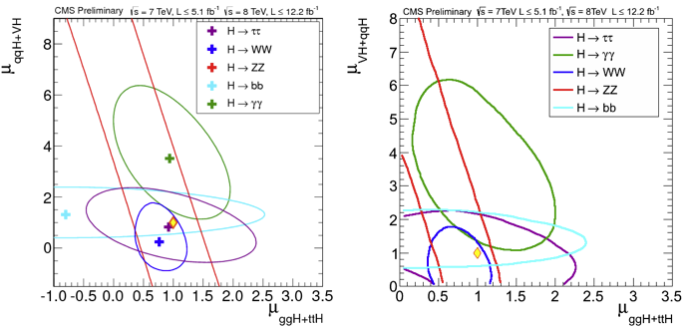
Fig. 62 (Left plot) The 68% CL intervals for signal strength in the gluon-gluon-fusion-plus-ttH and in VBF-plus-VH production mechanisms: \(\mu_{ggF + ttH}\) and \(\mu_{VBF+VH}\), respectively. The different colors show the results obtained by combining data from each of the five analyzed decay modes: \(\gamma\gamma\) (green), \(WW\) (blue), \(ZZ\)(red), \(\tau\tau\) (violet), \(bb\) (cyan). The crosses indicate the best-fit values. The diamond at (1,1) indicates the expected values for the SM Higgs boson. (right) The same intervals imposing the signal strength to be positive and computed using the Feldman-Cousins construction.

Underfluctuations and significance

The FC prescription, while giving a frequentist solution to several problems, it stumbles on a problem with eperiments having large background underfluctuations. Suppose you have two experiments:

• a super optimized experiment expects no background events and observes zero events in a given data taking period

• a less optimized experiment expects 10 background events and observes five events in a given data taking period

Using the FC prescription the upper limit on a signal at 90% CL for the first one is 2.44, while the second is 1.85. The worse experiment, clearly observing a lucky underfluctuation, obtains a better limit. This is not a desirable feature of the method. Quoting the authors: “The origin of these concerns lies in the natural tendency to want to interpret these results as the probability \(P(\mu|x_0)\) of a hypothesis given data, rather than what they are really related to, namely the probability \(P(x_0|\mu)\) of obtaining data given a hypothesis. It is the former that a scientist may want to know in order to make a decision, but the latter which classical confidence intervals relate to. […] scientists may make Bayesian inferences of \(P(\mu|x_0)\) based on experimental results combined with their personal, subjective prior probability distribution function. It is thus incumbent on the experimenter to provide information that will assist in this assessment.” The suggested way is to provide, together with the limit, also the sensitivity of the experiment, defined as “the average upper limit that would be obtained by an ensemble of experiments with the expected background and no true signal”. This extra information allows the reader to better understand if the value of a tight limit is just an artifact coming from an under-fluctuation of the background. When a significant portion of the upper limit curve is below the sensitivity of the experiment, the authors suggest to show both the sensitivity curve and the upper limit. Fig. 63

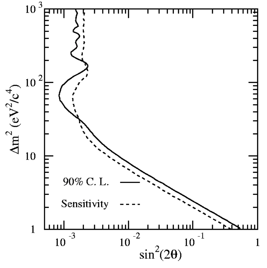
Fig. 63 Confidence region for an example of the toy model in which \(\sin^2(2\theta) = 0\) together with the sensitivity of the experiment.

LEP test statistic: \(L_{s+b}/L_b\)

To understand the test statistics \(L_{s+b}/L_b\) we will use as an example the search for the SM Higgs at LEP. Fig. 64 shows the Higgs candidate invariant mass distribution in data together with the histograms of the expected background and the expected signal at a mass of 115 GeV. The invariant mass is the discriminating variable used to extract the Higgs signal from background. We assume that, for each bin in invariant mass, we know what is the expected number of signal and background events. It is important to notice the difference between the invariant mass of a Higgs candidate \(m_H^{rec}\), which is the invariant mass computed from the reconstructed decay products and the test mass \(m_H\) which is the value of the mass at which we build the signal model we want to test.

The typical search for Higgs boson is a combination of the analyses of different Higgs production (at LEP mostly Higgsstrahlung and vector boson fusion) and decay modes (predominantly \(H\to b\bar{b}\) and \(H\to\tau^+\tau^-\)). The (extended) likelihood used for each production/decay mode is:

\[ L_{s+b} = \frac{(s(m_H)+b)^n}{n!}e^{-(s(m_H)+b)} \prod_{j=1}^{n_{bins}}\frac{s(m_H)S(x_j,m_H)+bB(x_j)}{s(m_H)+b} \]

which, for the background only hypothesis reduces to:

\[ L_{b} = \frac{b^n}{n!}e^{-b}\prod_{j=1}^{n_{bins}}B(x_j). \]

Here \(s\) is the number of expected signal events (which is a function of the test mass \(m_H\)), \(b\) the number of expected background events, \(n\) the number of observed events, \(x_j\) the value of the invariant mass \(m_H^{rec}\) (our discriminating variable) and \(S(x_j,m_H)\), \(B(x_j)\) the signal (function of the test mass) and background pdf computed at \(x_j\) (i.e. the signal and background shapes).

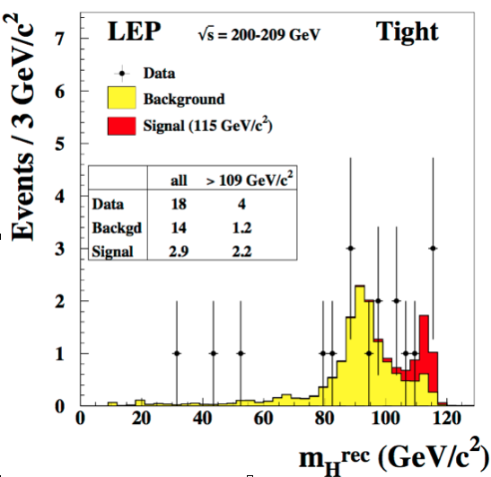
Fig. 64 Reconstructed invariant mass spectrum for the Higgs search at LEP.

The complete likelihood for the signal+background hypothesis is the product of the likelihoods of each production/decay:

(14)\[L_{s+b} = \prod_{k=1}^{N}\frac{(s_k(m_H)+b_k)^{n_k}}{n_k!}e^{-(s_k(m_H)+b_k)}\prod_{j=1}^{n^k_{bins}}\frac{s_k(m_H)S_k(x_{jk}; m_H)+b_kB_k(x_{jk})}{s_k(m_H)+b_k}\]

where the index \(k\) runs over the \(N\) production/decay modes analysed. The likelihood for the background only is trivially obtained again setting \(s\) to zero.

The discovery test statistics used at LEP is based on the likelihood ratio:

\[ Q = \frac{L_{s+b}}{L_b}. \]

Multiplying several positive numbers smaller than one, will quickly reach the machine numerical precision.

For the same numerical reasons already encountered for the likelihood, instead of Q, the logarithm of Q is used:

(15)\[q = -2 \ln Q = -2\ln\left(\frac{L_{s+b}}{L_b}\right).\]

Computing \(q\) explicitly with (14) we obtain:

\[ q = -2\ln Q(m_H) = 2\sum_{k=1}^{N}\left[ s_k(m_H) - \sum_{j=1}^{n^k_{bins}} \ln \left( 1+\frac{s_k(m_H)S_k(x_{jk}, m_H)}{b_k B_k(x_{jk})}\right)\right] \]

This expression shows that each bin contributes to the likelihood with a weight \(\ln(1+S/B)\) to the final test statistics. Because of this, a typical way to present the results is to plot the data as a function of \(\ln(1+s/b)\) as in Fig. 65. The region at large values of \(\ln(1+s/b)\) has the highest sensitivity to the signal.

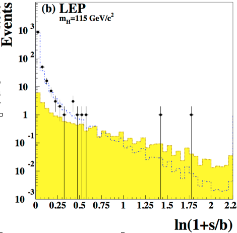
Fig. 65 Data (dots), signal (yellow histogram) and background (dashed histogram) as a function of \(\ln(1+s/b)\). In both cases the signal histogram is built for a test mass of 115 GeV.

The test statistic \(-2\ln(Q)\) is used to test for the presence of signal in data. The intuition goes as: compute the test statistics on the collected data and compare it with the “typical” test statistic values under the signal+background or background only hypotheses (see Fig. 66).

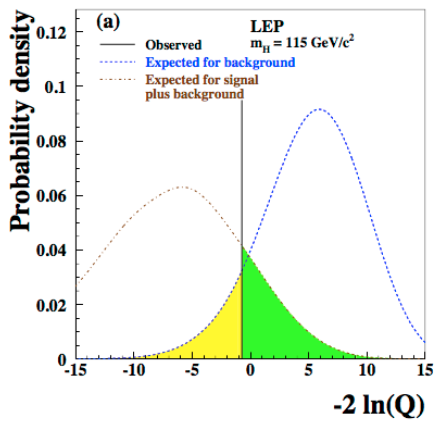
Fig. 66 Distribution of the test statistic \(-2\ln(Q)\) for the signal+background hypothesis in brown and background only hypothesis in blue. The value of the test statistic computed on data (observed) is represented by the vertical black line.

The “typical” values are obtained as the median of the pdf of the test statistic for the signal+background and the background only hypothesis. The pdfs are build from toy Monte Carlo samples. From the model in (14) we generate several toy datasets and for each of them we compute the test statistics \(-2\ln(Q)\). The blue and brown pdfs in Fig. 66 are the normalized histograms of the test statistics under the two hypothesis. To have a good estimation of the means, the histograms have to be well populated which means tossing a large number of toy experiments. This procedure is unfortunately very computing expensive. We will see later, when discussing the test statistics used at the LHC, how this problem can be mitigated. We can see from Fig. 66 that the pdf for the background only hypothesis clusters at large \(-2\ln(Q)\) values, while the signal+background at low values. The observed is somewhere in the middle and we will see in the next section how to use this value to set a limit on the Higgs boson production. Note that the values of the test statistic is a function of the test mass \(m_H\), in this plot the chosen value is \(m_H=115\) GeV. Scanning the value of the test mass we obtain Fig. 67. Here the median of the signal+background and the background-only hypotheses together with the observed value are plotted as curves (dashed brown and blue, and continuous black respectively) as a function of the test mass. The green(yellow) band covers the 68%(95%) area around the median of the background only hypothesis. These bands are a very common way to convey the statistical uncertainty of the background: presence of signal would appear in this plot as a deviation of the observed (black curve) from the expected for background only (dashed-blue); in absence of signal, the observed would be contained within the uncertainty bands. In Fig. 68 the same curves are plotted separately for each of the four LEP experiments (ALEPH, DELPHI, L3, OPAL). We see that for all experiments but ALEPH the observed fluctuates around the expected background only curve. ALEPH shows a signal-like fluctuation around 115 GeV.

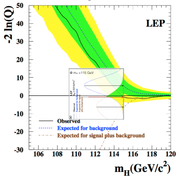
Fig. 67 Test statistics as a function of the test mass for the combined LEP experiments. The insert is Fig. 66 rotated and placed at the test mass of 115 GeV.

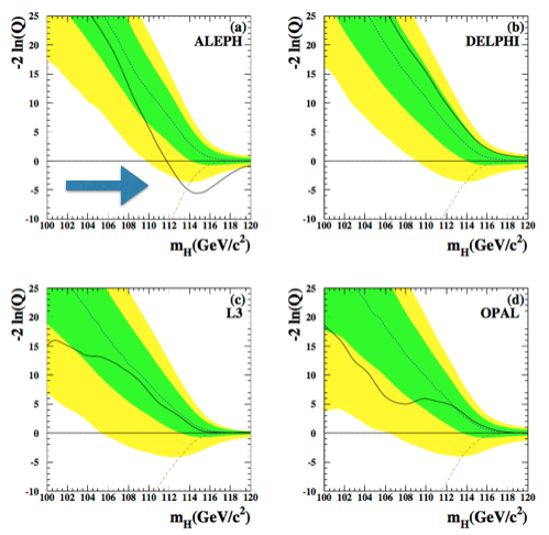
Fig. 68 Test statistics as a function of the test mass for the single LEP experiments.

To better characterize data fluctuations we can compute the already encountered \(p\)-value as the integral

(16)\[\int_{-\infty}^{-2\ln(Q_{obs})=q_{obs}}pdf(q|bkg)dq.\]

The smaller the \(p\)-value (the further out in the tail the \(q_{0,obs}\) lies), the poorest the agreement with the background only hypothesis. Conventionally if the \(p\)-value is below \(p = 2.87 \cdot 10^{-7}\), corresponding to a 5\(\sigma\) gaussian probability tail, we talk about “discovery”. Fig. 69 shows the \(p\)-value for the four LEP experiments combined and the separately for each of them. The ALEPH fluctuation observed in Fig. 68 corresponds to a \(p\)-value of \(\sim3~10^{-3}\) (i.e. \(\sim3\sigma\)), all other experiments are compatible with the background only hypothesis at that mass. The combined \(p\)-value shows a \(\sim2\sigma\) fluctuation around 95 GeV and a smaller one at around 115 GeV.

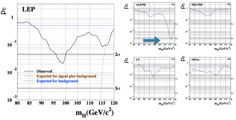
Fig. 69 p-values as a function of the test mass for the combined (left) and single (right) LEP experiments.

Nuisance parameters

FIXME: the only difference between a poi and nuisance parameters is that the latter has a constraint.

FIXME: add syst - nuisance - constraint gaussians, lognorm, flat

So far we have not considered any uncertainty on the signal and background models. Systematic uncertainties can arise from several sources and can affect both the signal (e.g. energy scale affecting the position of the signal, energy resolution affecting its width, etc…) and the background (the shape could come from some control region or sidebands, etc…). To include this uncertainties, we add more parameters to the model. These parameters are called nuisance parameters: \(\vec{\nu}\). For instance we can add an uncertainty \(\delta m\) on the mass position of the signal \(m_0\). The effect of these uncertainties is to widen the test statistics pdfs. The reason for this is rather intuitive, we are reducing the information in the model by including uncertainties on the parameters, and so the separation power between signal+background and background-only is reduced. The \(p\)-values will become a function also of these extra parameters, e.g.:

\[ \int_{-\infty}^{q_{obs}}\mbox{pdf}(q|m_0)dq \qquad\to\qquad\int_{-\infty}^{q_{obs}}\mbox{pdf}(q|m_0, \delta m)dq. \]

Ideally we would like any statement we make based on the pdf of the test statistics to be valid for any value of the nuisances. This turns out to be very restrictive when the values of the nuisance are disfavored by the data. At LEP a “hybrid frequentist-bayesian” procedure was followed to take into account nuisance parameters. Suppose you have a prior \(\pi(\nu)\) describing the degree of belief on where the nuisance parameter \(\nu\) lies. From the example above, the uncertainty on the mass scale could be constrained by calibration measurements to be gaussian distributed. Using the prior we can marginalize the likelihood:

\[ L_{\mbox{marginalized}} (x) = \int L(x|\nu) \pi(\nu) d\nu \]

and then proceed using this new likelihood to perform any frequentist test (\(p\)-value, intervals, etc…). The marginalization is usually done with Monte Carlo techniques, sampling the distribution \(\pi(\nu)\) and computing the likelihood at the sampled value \(\nu\).

The Neyman-Pearson lemma says that the likelihood ratio \(L_{s+b}/L_b\) for simple hypotheses is the optimal test statistics. The inclusion of nuisance parameters in the model changes the problem from the test of a simple hypothesis to a composite one, so strictly speaking the Neyman-Pearson lemma is not applicable. Nevertheless, when the nuisance parameters are well constrained, we can effectively consider the hypothesis to be simple and the likelihood ratio to be close to optimal.

The issue of sensitivity and the CLs procedure

The larger the expected signal the easier is to exclude it.

In absence of a clear signal observation (conventionally corresponding to a significance of \(3\sigma\)) we can still use our data to provide useful information about the largest signal we can exclude. We have already encountered the concept of upper limit in Sec.Confidence Belt. Let’s apply it to the Standard Model Higgs boson search at LEP. The search results were presented in terms of lower limits on the mass. The procedure to set the limit is straightforward. Look again at Fig. 66. In the previous section we used the observed value of the test statistics to define the \(p\)-value \(p_b\) on the pdf of the background only hypothesis (yellow area). This gave us the probability of the background to over-fluctuate to mimic a signal. Now we use the observed value of the test statistics to define the \(p\)-value \(p_{s+b}\) on the pdf of the signal+background hypothesis (green area).

Here we assuming that the searched for signal is the Standard Model Higgs boson, i.e. its production cross section/couplings/etc. are the ones predicted by the Standard Model.

This will give us the probability for the signal+background to under-fluctuate to mimic absence of signal. When \(p_{s+b} = 0.05\) we can exclude the presence of signal at the 95% CL. To set a limit on the mass of the SM Higgs boson we scan the values of the test mass until we find \(p_{s+b} = 0.05\).

In Fig. 70 we show the pdf of the test statistics for different test mass values. The central plot is again Fig. 66, the left one is computed at 110 GeV and the right one at 120 GeV. The lower the mass the larger the separation power between the signal+background and the background only hypothesis and this translates, for a given dataset, to lower and lower values of \(p_{s+b}\). We can read this as “given the expected SM-Higgs and the SM-backgrounds, it’s easier to exclude low mass values than high ones”. Going to high masses we see that the overlap between the two pdfs increases. The physical meaning of this is that we are not able anymore to separate the two hypothesis (in this case, we’re are reaching the kinematic limit of LEP to produce SM Higgs bosons).

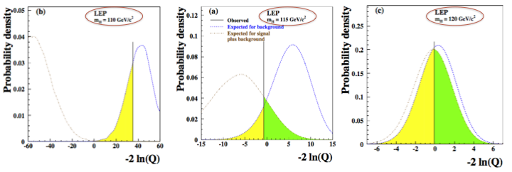
Fig. 70 The pdf of the test statistics for different test mass values.

This situation is rather dangerous. Let’s take a deeper look at the meaning of the \(p\)-values in Fig. 71 to understand why. The left plot focuses on the background only hypothesis: the right tail of the distribution contains experiments where the background under-fluctuates (i.e. we are lacking events also for the background only hypothesis), while the left tail instead contains the experiments where the backgroud over-fluctuates mimicking a signal. The right plot instead focuses on the signal+background hypothesis: the left tail contains experiments where the signal+background over-fluctuates, while in the right tail there are the under-fluctuations that mimic absence of signal.

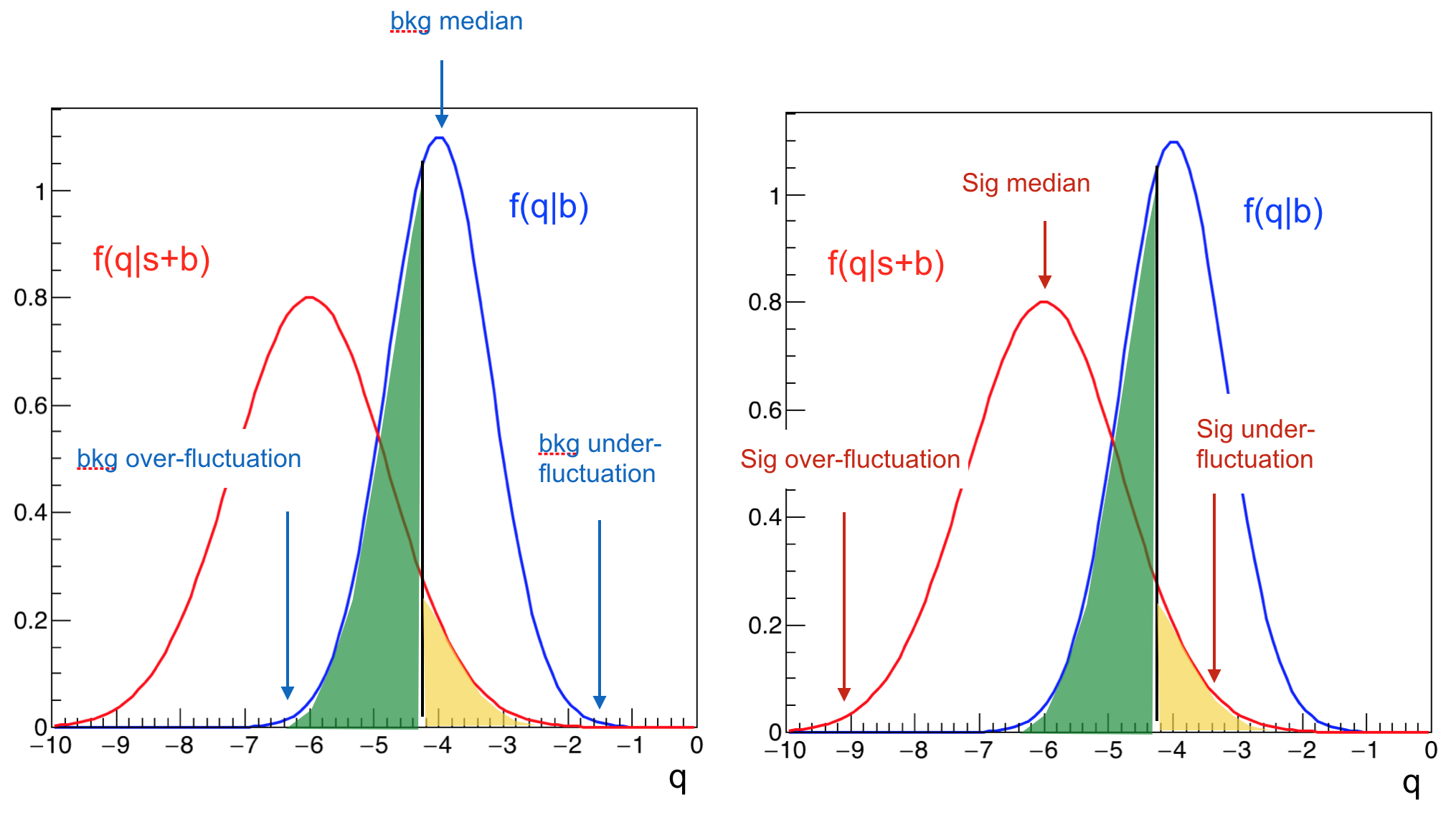
Fig. 71 Signal and background under/over fluctuations.

Let’s contrast this picture with Fig. 72. In this case the two pdfs largely overlaps providing very small separation power. Here is where the situation becomes dangerous. Suppose we are setting a 95% CL on a signal and the test mass used for Fig. 72 is the one providing \(p_{s+b} = 0.05\). In this case we can exclude the presence of a signal with such a mass at 95% CL, but we are also sitting on the right tail of the background. The background itself has an under-fluctuation! From the point of view of a signal search, it doesn’t make any sense. We are excluding the signal+background and the background-only hypotheses at the same CL. A situation like that could arise when trying to exclude a Higgs boson of 1 TeV at LEP where the kinematic reach is just above 100 GeV. While that is kinematically obvious, it is worth noticing that the procedure for limits settings detailed so far does not prevent to incur in such kind of troubles.

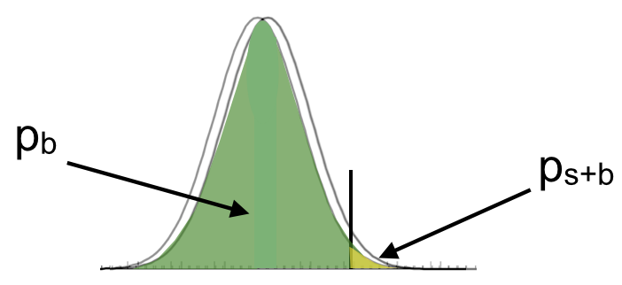
Fig. 72 Poor separation power.

This typically generate some confusion, the CL is a parameter set by hand and not a function of the data!

The root of the problem is that there is not enough information used in the limit setting procedure and we risk a “spurious exclusion”. A way to overcome this issue is to include somehow the information coming from \(p_b\). This is what the “CLs” procedure does. To illustrate the “CLs” procedure we will follow the notation of the original paper Ref.[Rea00]. The \(p_{s+b}\) is renamed “confidence level”. The confidence level of the signal+background hypothesis is then the integral \(CL_{s+b} = P(Q>Q_{obs}|s+b)\) calculated on the p.d.f. for signal+background hypothesis. Small values of \(CL_{s+b}\) correspond to a poor compatibility with the signal+background hypothesis and so favor the background only hypothesis and viceversa.

The idea stemmed from the frequentist approach of Zech to the problem of setting limits for a counting experiment in presence of background [@Zech].

The \(CL_s\) procedure “corrects” the \(CL_{s+b}\) dividing it by \(CL_b\), defined as \(CL_b = 1 - P(Q<Q_{obs}|b)\):

(17)\[CL_s = \frac{CL_{s+b}}{CL_b} = \frac{p_{s+b}}{1-p_b}\]

Remember that despite the misleading name, this is not a confidence level ! It’s not even a \(p\)-value, it’s a ratio of p-values. Nevertheless we will say that a signal is excluded at the confidence level CL if \(1-CL_s\ge CL\).

The false exclusion rate is now reduced:

• in case of a clear separation between the two hypothesis \(p_b\to 0\) and \(CL_s \to CL_{s+b}\), so we recover the standard p-value definition;

• in case of poor separation \(p_b \to 1\) and \(CL_s \to 1\), preventing spurious exclusions.

The results of the CLs procedure applied to the Higgs search at LEP are shown in Fig. 73. This is the famous plot excluding Higgs masses below 114.4 GeV [KT02].

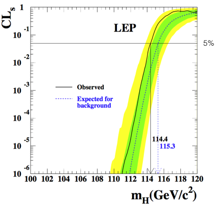
Fig. 73 LEP exclusion plot for the Standard Model Higgs search.

The CLs will deviate from the standard \(p\)-value the smaller the separation power of the test. The price to pay for this is that the limits obtained with the \(CL_s\) procedure will by construction “over-cover” resulting in conservative limits (you exclude less phase space). This is clearly not a desirable feature for a frequentist-based approach, but because “it works” it has been adopted as the standard way to set the limits at colliders. Opponents to this rather arbitrary procedure advocates the use of a Bayesian approach, which on the other hand raises the usual issues about setting a prior on the parameter under test.

For simplicity the CLs procedure has been detailed here using the LEP test statistics \(L_{s+b}/L_b\), but it can be applied precisely in the same way to the LHC test statistics that we will encounter in the next section.

LHC test statistics: \(-2\ln(\lambda(\mu))\)

In this section we describe the LHC test statistics and review the large sample approximations (Wald’s theorem and asymptotic formulas). We will develop the main concepts step by step using the discovery test statistic \(q_0\). Then we will develop the test statistic for upper limits and give some examples.

*In this section we will follow closely the paper in Ref. [CCGV11].

Profile likelihood ratio

Throughout this section we will use a concrete example to keep a uniform notation and help visualizing the results. For this “prototype experiment”, let’s assume that the data are represented by a histogram \(\textbf{n} = (n_1,\dots, n_N)\) in only one variable \(x\). For example x could be the candidate invariant mass (the generalization to several variables is trivial). The expected number of events in each bin of the histogram depends on our expectations of the signal and background:

\[ E[n_i]=\mu s_i + b_i \]

where:

• \(s_i\) is the number of signal events expected in bin \(i\): \(s_i = s_{tot} \int_{bin_i} f_s(x|\theta_s) dx\). The distribution \(f_s\) is the p.d.f. of the variable \(x\) for the signal, \(\theta_s\) are the parameters characterising the shape of the signal and \(s_{tot}\) is the total mean number of expected signal events;

• \(b_i\) is the number of background events expected in bin \(i\): \(b_i = b_{tot} \int_{bin_i} f_b(x|\theta_b)dx\). The distribution \(f_b\) is the p.d.f. of the variable \(x\) for the background, \(\theta_b\) are the parameters characterising the shape of the background and \(b_{tot}\) is the total mean number of expected background events.

• the parameter \(\mu\) is the signal strength that we have already encountered and which allows to go in a continuous way from the background only hypothesis \(\mu=0\) to the nominal signal+background hypothesis \(\mu=1\)

We group all parameters, but the signal strength \(\mu\) our parameter of interest, in a vector \(\vec{\theta}=(\theta_s,\theta_b,s_{tot},b_{tot})\) of nuisance parameters.

You want to extract the fraction of signal events in a data sample \(D\). The statistical model used is:

\[ L(D|f_{sig}) = f_{sig}~\mbox{Gauss}(m;m_0,\sigma) + (1-f_{sig})~e^{-\alpha m} \]

where the observable \(m\) is the invariant mass of the candidates, \(f_{sig}\) is the fraction of signal events, \(m_0\) is the position of the resonance, \(\sigma\) is the width of the resonance and \(\alpha\) is the slope of the background. The parameter of interest is \(f_{sig}\), all the other parameters of the model are \(\vec{\theta}=\{m_0,~\sigma,~\alpha\}\).

Typically in a measurement, together with the main dataset, we use several other samples to help constraining the parameters of the model (e.g. the background in the signal region can be constrained by the measurement of the number of events in a control sample). These constraints are usually collected in auxiliary histograms \(\textbf{m} = (m_1, \ldots, m_M)\):

\[ E[m_i] = u_i(\theta) \]

where the \(u_i\) are quantities that depend on \(\theta\) and model e.g. the shape of the background. With this we can build the complete likelihood used to model the data:

\[ L(\mu,\theta) = \prod_{j=1}^{N} \frac{(\mu s_j + b_j)^{n_j}}{n_j!} e^{-(\mu s_j + b_j)} \prod_{k=1}^{M} \frac{u_k^{m_k}}{m_k!} e^{-u_k}. \]

The test statistic developed at the LHC is based on a profile likelihood ratio defined by:

(18)\[\lambda(\mu) = \frac{L(\mu,\hat{\hat{\theta}})}{L(\hat{\mu},\hat{\theta})}\]

where:

• \(\mu\) is the value we are testing

• \(\hat{\hat{\theta}}\) is the best fit of the nuisance parameters once we fixed the \(\mu\) we want to test (i.e. conditional to the test value \(\mu\) in the likelihood). We say in this case that the parameters \(\theta\) are profiled. The value of \(\hat{\hat{\theta}}\) is a function of \(\mu\).

• \(\hat{\mu}\) and \(\hat{\theta}\) are the best fit values of \(\mu\) and \(\theta\) (the parameter of interest and the nuisances) when both are left floating in the likelihood. In other words \(\hat{\mu}\) and \(\hat{\theta}\) are the values that maximize the likelihood.

The denominator of this ratio is just a likelihood function, the numerator is called “profile likelihood” and the ratio is called “profile likelihood ratio”. The fitted value \(\hat{\mu}\) is allowed to take any positive or negative (unphysical) values (provided that \(\mu s_i + b_i\) in the Poisson remains positive) even in the case where the search targets a positive signal. This assumption, rather arbitrary at this point, will be needed in the following to model \(\hat{\mu}\) as a gaussian distributed variable, that will allow write the test statistics in an analytical closed form.
The values taken by the profile likelihood ratio \(\lambda(\mu)\) are in the interval \([0,1]\). The ratio will get to unity the closer the test value of \(\mu\) is to the value of \(\hat{\mu}\) preferred by the data. On the contrary it will approach zero for test values of \(\mu\) very different from \(\hat{\mu}\).
As already noticed for the LEP test statistics, the inclusion of nuisance parameters changes the hypothesis under test from simple to composite. Generally, however, the nuisance parameters are well constrained and the likelihood ratio test is close to optimal. The inclusion of the nuisance parameters should give enough flexibility to the likelihood to be able to model the “true” unknown values of the parameters. Ideally, when making statements based on a test statistics (e.g. when setting a limit on \(\mu\) at \(1-\alpha\) level) we would like it to be correct for all values of the nuisances. In general it is not possible to cover all values of the nuisances and as consequence the coverage is not guaranteed. Nevertheless the choice of a profile likelihood ratio allows to have the correct coverage at least in a “trajectory” given by \((\mu, \hat{\hat{\theta}})\) [Cra08].

Discovery test statistics

From the definition in Eq.(18) we can build several test statistics. Instead of listing all of them, let’s learn how to use one and come back later to some of the other cases. We will start from the discovery test statistics for a positive signal; this is the typical case for searches at the LHC. We want to test for \(\mu=0\) which correspond to the background only hypothesis. Rejecting the background only hypothesis corresponds to acknowledge the presence of something else in data which is not described correctly: a signal. The discovery test statistics for positive signals is defined as:

(19)\[\begin{split} q_0 = \left\{ \begin{array}{rll} -2 \ln \lambda(0) & \mbox{if} & \hat{\mu} \ge 0 \\ 0 & \mbox{if} & \hat{\mu} < 0 \end{array}\right.\end{split}\]

where \(\lambda(0)\) is the is the profile likelihood ratio for \(\mu = 0\) as defined in Eq.(18). With this definition, large values of \(q_0\) correspond to increasing incompatibility between the data and the background only hypothesis. Remember that \(\mu\) is the value you are testing, in this case \(\mu=0\), while \(\hat{\mu}\) is the value you fit from data (the so called “best fit”). The idea to have different definitions for positive and negative values of \(\hat{\mu}\) has a simple explanation. If the measured value \(\hat{\mu}\) is negative, it means that we are observing fewer events than what we would expect from the background only hypothesis. In absence of signal, that should happen 50% of the times: for large enough statistics allowing for a gaussian description, 50% of the times the background fluctuates up, 50% it fluctuates down. Under-fluctuations of the background are of no interest for the search of an excess of events in data. To discover a new signal we are only interested in upper fluctuations of data with little compatibility with the background only model, i.e. \(\hat{\mu} \ge 0\).
To quantify the level of disagreement between the background only hypothesis and the observed value of the test statistics, we can compute the \(p\)-value

\[ p=\int_{q_{0,obs}}^\infty f(q_0|0) dq_0 \]

\(f(q_0|0)\) denotes the pdf of the statistic \(q_0\) under assumption of the background-only (\(\mu = 0\)) hypothesis (see Fig. 74). Note that the extremes of the \(p\)-value integral are different from the LEP case in Eq.(16) because of the different test statistics definition.

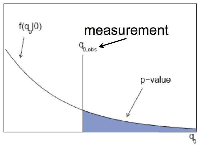
Fig. 74 Example of a measured p-value when having the observed test statistics \(q_{0,obs}\). Good compatibility with \(H_{0}\) corresponds to a \(q_{0,obs}\) which is on the left side (i.e. has a large p-value), whereas a \(q_{0,obs}\) on the far right indicates bad compatibility.

In order to compute the integral we need to know \(f(q_0|0)\). The brute force way to build the p.d.f. for the test statistics \(q_0\) is through toy experiments. Each toy experiment is created by generating random data on the background only model; to be representative of the luminosity in the data set we are analysing, the number of events in each toy has to match the one of the measured data sample. For each toy we then compute the test statistics and fill a histogram. The number of toy experiments to be generated depends on the significance we are trying to estimate. Because the \(p\)-value is computed by integrating the histogram above \(q_{0,obs}\), we will need to properly populate the tail of the distribution above \(q_{0,obs}\). To quantify a deviation corresponding to a discovery (\(2.87 \cdot 10^{-7}\)) we will need to generate a number of toy experiments significantly larger than \(1/(2.87 \cdot 10^{-7})\)

Example:

Suppose you want to estimate the \(p\)-value for the measured test statistics \(q_{0,obs}\) where the signal appears in the distribution of the invariant mass as gaussian bump on an exponentially falling background. The procedure is depicted in Fig. 75. From the exponential distribution describing the background we generate random events following e.g. the “hit or miss” method shown in Sec. MC. The number of events to be generated has to be same as the one experimentally collected (i.e. representing the same integrated luminosity). We repeat the data generation a large number of times, we compute the test statistics for each “toy experiment” and fill a histogram with those values. The observed \(p\)-value is simply the integral of the histogram from \(q_{0,obs}\) to infinity.

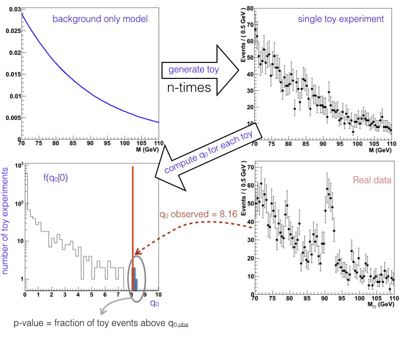
Fig. 75 Cartoon showing how to extract the \(p\)-value from a toy study. The pdf \(f(q_0|0)\) is approximated by the histogram normalized to unit area.

Asymptotic Formulas

So far we have seen how to build the test statistics \(f(q_0|0)\) tossing toy experiments and how CPU expensive that is. In recent years Cowan at al. in Ref. [CCGV11] have used results proved by Wilks and Wald in the early ’40s to overcome this problem and find an analytic formula to describe the generic pdf \(f(q_\mu|\mu')\).

The Wald’s theorem basically states that in the limit of a sufficiently large data sample we can approximate the test statistics \(-2\ln\lambda(\mu)\) (see Eq.(18)) as:

(20)\[-2\ln\lambda(\mu) = \frac{(\mu-\hat{\mu})^2}{\sigma^2} + o\left( \frac{1}{\sqrt{N}}\right)\]

where \(\mu\) is the value we are testing, \(\hat{\mu}\) is the estimator of \(\mu\) and the width \(\sigma\) can be extracted from the second derivative of the likelihood (Fisher information) as

\[ V^{-1}_{ij} = -E\left[ \frac{\partial^2 \ln L}{\partial \theta_i \partial \theta_j} \right] \]

or using the Asimov dataset that we will describe in the next section.
The importance of Wald’s theorem is that, for large enough statistics, the estimator \(\hat{\mu}\) is gaussian distributed around \(\mu'\) (the true value of the parameter \(\mu\) - unknown in data, only nature knows it, or known in a Monte Carlo sample, you decided its value) and that all the parameters of the gaussian distribution can be computed. The “large enough” sample limitation is needed to be able to neglect the term \(o\left( \frac{1}{\sqrt{N}}\right)\), but we will see later that the approximation is valid for relatively low number of events.
Neglecting the term \(o(1\sqrt{N})\) the test statistics \(t_{\mu} = -2\ln \lambda({\mu})\) is distributed as a “non-central \(\chi^2\)” distribution for one degree of freedom.

\[ f(t_\mu|\Lambda) = \frac{1}{2\sqrt{t_\mu}}\frac{1}{\sqrt{2\pi}}\left[ \exp \left( -\frac{1}{2} (\sqrt{t_\mu} + \sqrt{\Lambda})^2 \right) + \exp\left( -\frac{1}{2} (\sqrt{t_\mu} - \sqrt{\Lambda})^2 \right) \right] \]

with the non-centrality parameter \(\Lambda\)

\[ \Lambda = \frac{(\mu-\mu')^2}{\sigma^2} \]

The Wilks’ theorem is a special case of the Wald’s theorem for \(\mu'=\mu\), \(\Lambda = 0\). In that case \(-2\ln\lambda(\mu)\) approaches a \(\chi^2\) distribution for one degree of freedom.

We can now apply these results to the discovery test statistics. In the approximation of large test statistics Eq.(20):

(21)\[\begin{split} q_0 = \left\{ \begin{array}{rll} -2 \ln \lambda(0) & \mbox{if} & \hat{\mu} \ge 0 \\ 0 & \mbox{if} & \hat{\mu} < 0 \end{array}\right. \qquad \Rightarrow \qquad q_0 = \left\{ \begin{array}{rll} \hat{\mu}^2/\sigma^2 & \mbox{if} & \hat{\mu} \ge 0 \\ 0 & \mbox{if} & \hat{\mu} < 0 \end{array}\right. \end{split}\]

where the estimator \(\hat{\mu}\) is gaussian distributed around the mean \(\mu'\). The pdf for the test statistics for a generic \(\mu'\) becomes:

(22)\[f(q_0|\mu') = \left( 1-\Phi\left(\frac{\mu'}{\sigma} \right)\right)\delta(q_0) + \frac{1}{2}\frac{1}{\sqrt{2\pi}}\frac{1}{\sqrt{q_0}} \exp\left[-\frac{1}{2}\left(\sqrt{q_0} - \frac{\mu'}{\sigma} \right)^2\right]\]

The special case where \(\mu'=0\) , i.e. in the hypothesis of background only, this equation simplifies to

(23)\[f(q_0|0) = \frac{1}{2}\delta(q_0) + \frac{1}{2}\frac{1}{\sqrt{2\pi}}\frac{1}{\sqrt{q_0}} e^{-\frac{q_0}{2}}\]

Compare this formula to the bottom left plot in Fig. 75. The delta function describes the first bin of the histogram; this comes from our choice to set the test statistics to zero when \(\hat{\mu}<0\). The coefficient 1/2 of the delta function reflects the 50% probability of the background to fluctuated below zero. The exponentially falling part instead describes the tail of distribution for \(\hat{\mu}>0\).
To get to the \(p\)-value using toys, we had to integrate the histogram above the observed value of the test statistics. In the approximation of large sample, using Wald’s theorem, this corresponds to the integral of Eq.(23) above the observed value of the test statistics. The simple form of the pdf gives an even simpler expression for the cumulative of Eq.(22)

\[ F(q_0|\mu') = \Phi\left( \sqrt{q_0} - \frac{\mu'}{\sigma} \right) \]

which, for \(\mu'=0\) as in Eq.(23), becomes:

\[ F(q_0|0) = \Phi\left( \sqrt{q_0} \right). \]

The \(p\)-value can them be simply computed as $\(p_0 = 1-F(q_0|0)\)$ obtaining for the significance

\[ Z_0 = \Phi^{-1}(1-p_0) = \sqrt{q_0}. \]

The signal significance is simply the square root of the observed test statistics! To fully appreciate this result, think about the evaluation of the significance for a \(5\sigma\) signal: using toys you need to produce \(o(10^8)\) data samples to populate the high tail of \(f(q_0|0)\) to compute the integral above \(q_0^{obs}\) (and then convert it to a significance); with the asymptotic to get you just take the square root of \(q_0^{obs}\): if \(q_0^{obs} = 25\) you have a \(5\sigma\) deviation!

Example:

Fig. 76 shows the scan of the test statistics as a function of \(\mu\). The minimum is obtained when \(\hat{\mu} = \mu\) and it is zero by construction of the likelihood ratio. The intercept at \(\mu=0\) i.e. \(q_0^{obs} = -2\ln(\lambda(0))\) is the square of the significance. This means that we can read off the vertical axis the significance of the signal as \(\sqrt{14.25} = 3.8\sigma\).

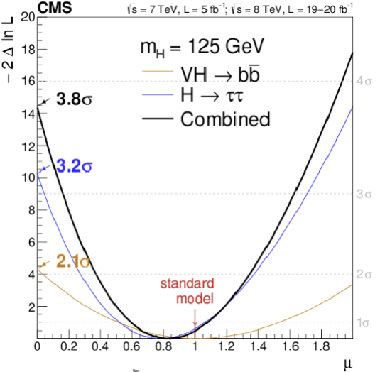
Fig. 76 Observation of the Higgs coupling to fermions.

Example:

Fig. 77 shows results of the \(H\to\gamma\gamma\) search at CMS using the \(p\)-value computed at each test mass hypothesis. The black continuous line is the observed \(p\)-value, that is computed on the asymptotic pdf for \(f(q_0|0)\) using the measured \(q_0^{obs}\), the dashed black line represent the expected \(p\)-value for the Standard Model signal (\(\mu=1\)). The other curves represent the observe and expected \(p\)-values for different datasets collected by CMS at the LHC with different centre of mass energies (\(\sqrt{s}=7\) TeV and \(\sqrt{s}=8\) TeV).

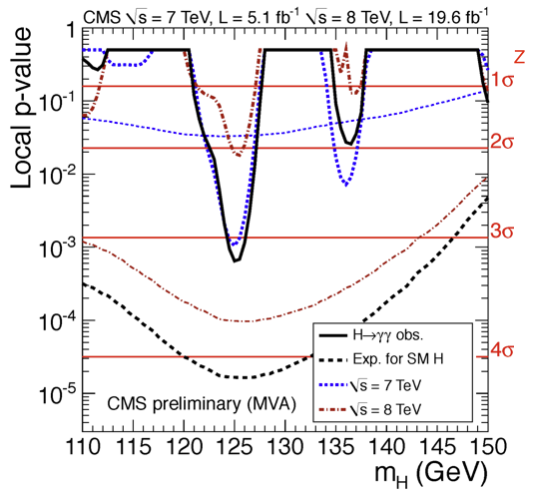
Fig. 77 Expected (dashed) and observed (continuous) \(p\)-values for the CMS \(H\to\gamma\gamma\) search. The red curves are computed on the first data collected in 2011, the blue ones for the data collected in 2012 and the black curves on the two data set combined.

Asimov dataset

There are cases where you want to have the estimation of the expected significance of a signal. Typically this happens during the design phase of an experiment or, after a measurement, when you want to compare the observed and expected significances. To do this you need to have access to two pdfs: \(f(q_0|0)\), the distribution of the test statistics in the background only hypothesis and \(f(q_0|1)\), the distribution of the test statistics in the signal+background hypothesis. In the latter case \(\mu=1\) indicates the expected value of the signal strength. A sketch of these two functions is shown in Fig. 78.

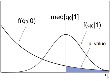
Fig. 78 Discovery statistics distribution under the background only \(f(q_0|0)\) and signal + background \(f(q_0|1)\).

We have already encountered above the pdf \(f(q_0|0)\): the most probable value of the test statistic is zero and the large tail corresponds to signal-like fluctuation of the background only hypothesis. The pdf \(f(q_0|1)\) instead clusters at high values of \(q_0\). We can understand this from the definition of the likelihood ratio \(\lambda(0) = L(0, \hat{\hat{\theta}})/L(\hat{\mu},\hat{\theta})\). Here \(\hat{\mu} = 1\) by construction, so the ratio \(\lambda(0)\) will cluster around small values of the test statistics and consequently \(-2\ln(\lambda(0))\) will cluster at large ones.

To compute the expected significance of a signal, we compute the \(p\)-value as the integral from the median of the \(f(q_0|1)\) distribution to infinity. We use the median as the “most representative” value for the expected signal+background.

The name comes from the short story “Franchise” from I. Asimov, where in the far future of 2008 the U.S.A. elections were to be replaced by the choice of a single citizen chosen by a computer which would represent the perfect average of the whole population

To compute the median value of the test statistics we first need the pdf from toys or the asymptotic formulas. Can we produce a single dataset such that if we compute the test statistics on it we get the median value of the pdf ? This is the idea behind the “Asimov” dataset. This can be thought as “the perfect average” of the experiments outcome. To understand how to build this dataset, we can use the prototype analysis:

\[ L(\mu,\theta) = \prod_{j=1}^{N} \frac{(\mu s_j + b_j)^{n_j}}{n_j!} e^{-(\mu s_j + b_j)} \prod_{k=1}^{M} \frac{u_k^{m_k}}{m_k!} e^{-u_k} \]

From here we can find the ML estimator for the parameters as

\[ \frac{\partial \ln L}{\partial \theta_j} = \sum_{i=1}^{N} \left( \frac{n_i}{\nu_i}-1 \right) \frac{\partial \nu_i}{\partial \theta_i} + \sum_{i=1}^{M}\left( \frac{m_i}{u_i} -1 \right) \frac{\partial u_i}{\partial \theta_j} = 0 \]

and define the Asimov dataset bin by bin as:

\[\begin{split} \begin{aligned} n_{i,A} &=& E[n_i] = \nu_i = \mu' s_i(\theta) + b_i(\theta)\\ m_{i,A} &=& E[m_i] = u_i(\theta).\end{aligned} \end{split}\]

Each bin of the Asimov dataset has by construction the number of entries equal to the expected value, with the correct statistical uncertainty. The only difference with respect to a toy data set is that there are no statistical fluctuation associated to the entries per bin.
On the Asimov dataset we can compute the Asimov likelihood and use it to compute the likelihood ratio:

\[ \lambda_A(\mu) = \frac{L_A(\mu, \hat{\hat{\theta}})}{L_A(\hat{\mu},\hat{\theta})} \sim \frac{L_A(\mu, \hat{\hat{\theta}})}{L_A(\mu',\theta)} \]

where by construction of the Asimov, \(\hat{\mu}=\mu'\) and the nuisance parameters \(\hat{\theta}=\theta\).

The Asimov can also be used to obtain the width \(\sigma\) for the approximate formula in Eq.(20):

\[ q_\mu = -2\ln\lambda(\mu) = \frac{(\mu-\hat{\mu})^2}{\sigma^2} + o\left( \frac{1}{\sqrt{N}}\right) \qquad\Rightarrow\qquad q_{\mu,A} = -2\ln\lambda_A(\mu) \sim \frac{(\mu -\mu')^2}{\sigma^2}. \]

From here we can extract

\[ \sigma_A^2 = \frac{(\mu - \mu')^2}{q_{\mu,A}} \]

Finally, it’s easy to verify that the test statistic computed on the Asimov dataset coincides with the median of the distribution \(f(q_\mu|\mu')\):

\[ \mbox{med}[q_0] = q_0(\mbox{med}[\hat{\mu}]) = \frac{\mu'}{\sigma} = -2\ln \lambda_A(0) \]

where the first equality comes from the fact that the median of the \(q_0\) is the value of \(q_0\) computed at the median value of \(\hat{\mu}\), the second equality comes by construction of the Asimov dataset \(\mbox{med}[\hat{\mu}] = \mu'\), \(q_0(\mu') = (0-\mu')^2/\sigma^2\) and the last one comes from the Wald’s theorem in Eq.(21). The expected significance \(Z_0 = \sqrt{q_0}\) computed on the Asimov dataset is then simply \(\mbox{med}[Z_0] = \sqrt{-2\ln\lambda_A(0)}\).

Upper limits test statistic

To set an upper limit we can define the following test statistics:

\[\begin{split} q_\mu = \left\{ \begin{array}{rll} -2 \ln \lambda(\mu) & \mbox{if} & \hat{\mu} \le \mu \\ 0 & \mbox{if} & \hat{\mu} > \mu \end{array}\right. \end{split}\]

Here we are using the same profile likelihood ratio as for the discovery test statistics, but this time we test for a generic \(\mu\). Notice that that is not the only difference in the definition. The \(\le\) and \(>\) signs are swapped with respect to Eq.(19). The reason for this is that, given that we are only considering cases where signal is associated to an excess of events above the background, we can only exclude an hypothesised value of \(\mu\) if the observed \(\hat{\mu}\) fluctuates below that. Vice versa, we cannot exclude a value of \(\mu\) if the observed \(\hat{\mu}\) is measured above the tested value \(\mu\) and so we set the test statistics to zero.

As we have already done for the discovery test statistics we can define a \(p\)-value as:

\[ p_\mu = \int_{q_{\mu,obs}}^\infty f(q_\mu|\mu)dq_\mu \]

How do we set a upper limit with this test statistics? Suppose you want to set an upper limit at 95% CL. You need to scan the values of \(\mu\) until you find the largest value of \(\mu\) such that the \(p\)-value is equal to 0.05. Practically you will also need to guess what is the range of \(\mu\) values to scan and what step to use in the scan.
 To set the expected upper limit on the signal strength of a signal you need first to get the pdf for \(f(q_\mu|\mu')\). Analogous to what we have seen with the discovery test statistics the distributions for \(\mu'=\mu\) and \(\mu'\neq\mu\) are as shown in Fig. 79. In particular we will need the pdf \(f(q_\mu|0)\) describing the test statistics in absence of signal, from which we extract the median value, and then scan the values of \(\mu\) (same procedure used for the observed) until you find the largest value of \(\mu\) such that the \(p\)-value is equal to the desired \(\alpha\)=1-CL.

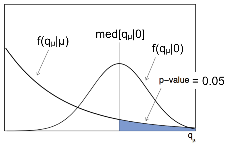
Fig. 79 Sketch of the pdf for \(f(q_\mu|\mu')\).

Very often when displaying the expected upper limits we also show the 1\(\sigma\) and 2\(\sigma\) uncertainty bands around the expected median. To do this, from the median value (i.e. 50% quantile) of the distribution giving the desired \(\alpha\) = 1-CL, i.e. med\([q_\mu|0]\), we can quote the “median\(\pm 1 \sigma\)” (16%, 84% quantiles), and the “median\(\pm 2 \sigma\)” (5%, 95% quantiles), as shown in Fig. 80.

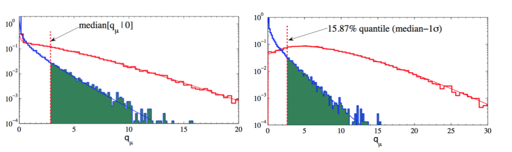
Fig. 80 Median (50% quantile) and median \(-1\sigma\) (15.87% quantile).

The observed limits together with the expected one and its respective uncertainty bands are shown as a function of the test mass in Fig. 81.

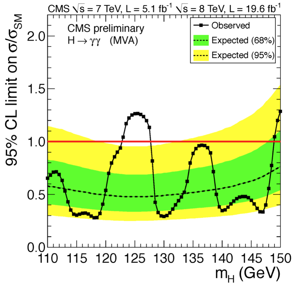
Fig. 81 Describe the red line as SM limit.

Using Wald’s theorem the asymptotic formula for the test statistic becomes:

\[\begin{split} q_\mu = \left\{ \begin{array}{rll} -2 \ln \lambda(\mu) & \mbox{if} & \hat{\mu} \le \mu \\ 0 & \mbox{if} & \hat{\mu} > \mu \end{array}\right. \qquad \Rightarrow \qquad q_\mu = \left\{ \begin{array}{rll} \frac{(\mu-\hat{\mu})^2}{\sigma^2}& \mbox{if} & \hat{\mu} \le \mu \\ 0 & \mbox{if} & \hat{\mu} > \mu \end{array}\right. \end{split}\]

where \(\hat{\mu}\) is, as for the discovery test statistics, gaussian distributed around \(\mu'\) with standard deviation \(\sigma\). From this expression, it is possible to compute the closed form expression for \(f(q_\mu|\mu')\):

\[ f(q_\mu|\mu') = \Phi\left(\frac{\mu' - \mu}{\sigma} \right)\delta(q_\mu) + \frac{1}{2}\frac{1}{\sqrt{2\pi}}\frac{1}{\sqrt{q_\mu}} \exp\left[-\frac{1}{2}\left(\sqrt{q_\mu} - \frac{\mu-\mu'}{\sigma} \right)^2\right] \]

which, for the special case where \(\mu = \mu'\), becomes:

\[ f(q_\mu|\mu) = \frac{1}{2}\delta(q_\mu) + \frac{1}{2}\frac{1}{\sqrt{2\pi}}\frac{1}{\sqrt{q_\mu}} e^{-\frac{q_\mu}{2}} \]

Using the cumulative distribution \(F(q_\mu|\mu') = \Phi\left(\sqrt{q_\mu}-\frac{\mu - \mu'}{\sigma}\right)\) we get \(p_\mu = 1-F(q_\mu|\mu') = 1 - \Phi(\sqrt{q_\mu})\), which, as for the discovery test statistic, gives:

\[ Z_\mu = \Phi^{-1}(1-p_\mu)=\sqrt{q_\mu} \]

The upper limit at \((1-\alpha)\) CL on \(\mu\) is the largest value of \(\mu\) such that \(p_\mu\leq \alpha\). With the asymptotic formulas we just need to set \(p_\mu = \alpha\) and solve \(\mu_{up} = \hat{\mu} + \sigma\Phi^{-1}(1-\alpha)\).

Combining measurements

As we have already seen in Sec.Likelihood:Combining measurements, the results of different measurements of a given parameter \(\mu\) can easily be combined by multiplying their likelihoods:

\[ L(\mu,\vec{\theta}) = \prod_i L_i(\mu, \vec{\theta}_i) \]

where the subscript \(i\) stands for the different experiments (e.g. ATLAS, CMS) or different processes (e.g. \(H\to \gamma\gamma\), \(H\to ZZ\), etc…).

Whenever different measurements are combined we need to pay attention at the possible correlations between the nuisances among the different experiments/channels. Typically the nuisances are chosen to be:

• uncorrelated: we use different parameters in the likelihoods of the different experiments to describe the nuisance

• fully correlated: we use the same parameter in all the likelihoods to describe the nuisance

• fully anticorrelated: we use again one parameter but we flip its sign.

To compute the expected significance for the combination the easiest approach is to use the Asimov dataset:

\[ \lambda_A(\mu) = \prod_i \lambda_{A,i}(\mu) \qquad \mbox{where}\qquad \lambda_{A,i}(\mu) = \frac{L_{A,i}(\mu, \hat{\hat{\theta}})}{L_{A,i}(\hat{\mu},\hat{\theta})} = \frac{L_{A,i}(\mu, \hat{\hat{\theta}})}{L_{A,i}(\hat{\mu'},\hat{\theta})}. \]

where the last equality comes from the properties of the Asimov dataset (\(\hat{\mu}\) converges by construction to \(\mu'\)).

Discovery significance: \(S/\sqrt{B}\)

Consider a counting experiment where you observe \(n\) events, the expected number of background events is \(b\) and the expected number of events in case of signal is \(s+b\). To simplify let’s first consider the case of large statistics such that the we can approximate the Poisson distribution with a Gaussian \(G(x|\mu, \sigma)\) with \(\mu = s+b\) and \(\sigma = \sqrt{s+b}\) (the fact that the n is a discrete variable, wile x is continuous is irrelevant in this context).

The significance to reject the background hypothesis can be quantified as the \(p\)-value associated to the observation of \(x\) events Prob\((x>x_{obs} | s = 0)\) which, for a gaussian, is simply \(p_0 = 1-\Phi((x_{obs}-b)/\sqrt{b})\). The significance is then \(Z_0 = \Phi^{-1}(1-p_0) = (x_{obs} - b)/\sqrt(b)\).

The median significance to for a signal \(s\neq0\) can be computed in the same way replacing \(x_{obs}\) with the median signal plus background i.e. \(s+b\):

\[ \mbox{median}[Z_0 | s+b] = \frac{s+b-b}{\sqrt{b}} = \frac{s}{\sqrt{b}} \]

giving the famous formula for the the signal significance. This is the typical quantity we try to maximize when optimizing a selection in a search.
This formula is only valid in the limit of large statistics. For the most general case we need to go back to the Poisson distribution:

\[ L(n|s+b) = \mbox{Poisson}(n|s+b) = \frac{(s+b)^n e^{-(s+b)}}{n!} \]

or taking the logarithm

\[ \ln L(n|s+b) = n\ln(s+b) -(s+b) -\ln n! \]

Recalling that the ML estimator for \(s\) is simply \(\hat{s} = n-b\), we can build the test statistic:

\[\begin{split} q_0 = \left\{ \begin{array}{lll} -2 \ln \lambda(0) = -2\ln \frac{L(n|0+\hat{b})}{L(n|\hat{s}+\hat{b})} = 2( n \ln \frac{n}{b} + b -n) & \mbox{if} & n > b \\ 0 & \mbox{if} & n \leq b \end{array}\right. \end{split}\]

Now we can use Wald’s theorem and rewrite the significance to reject the background only hypothesis as:

\[\begin{split} Z_0 \sim \left\{ \begin{array}{lll} \sqrt{q_0} = \sqrt{2( n \ln \frac{n}{b} + b -n)} & \mbox{if} & n > b \\ 0 & \mbox{if} & n \leq b \end{array}\right. \end{split}\]

The median significance from the expected signal plus background \(s+b\) is:

\[ \mbox{median}[Z_0 | s+b] = \sqrt{2( (s+b) \ln (s/b +1) -s)}. \]

This formula can be considered as a generalization of \(s/\sqrt{b}\). If we expand this result to the second order in the limit of \(s << b\) we get back to \(s/\sqrt{b}\). This is an important condition to keep in mind when using \(s/\sqrt{b}\). If \(s\) and \(b\) are both large, then the \(p\)-value goes to zero! The \(p\)-value is the probability to observe a fluctuation as large or larger than the one observed, if both \(s\) and \(b\) are large that probability is vanishingly small.

Examples from the search of the Higgs at the LHC

In this section we will walk through some results from search for the Higgs boson at the LHC, taking the \(H\to \gamma\gamma\) as the conceptually easy example of a search of a “bump” on top of a falling background. All plots are taken from the public CMS results [CMS]

Best fit signal strength

The plot in Fig. 82 shows the best fit of the signal strength modifier \(\hat{\mu}\) as a function of the test mass \(m_H\). The value obtained fluctuates around \(\hat{\mu}\sim 0\) everywhere in but in the region around 125 GeV where the excess was observed in the exclusion limits (Fig. 81) and in the \(p\)-value plot in Fig. 77. In that region, the signal strength steeply raise to a value compatible with the Standard Model expectation of \(\mu=1\). The green band represent the uncertainty on \(\hat{\mu}\) defined on the likelihood ratio as \(-2\ln \lambda(\mu) = -2 \ln L(\mu) / L(\hat{\mu}) <1\) which is equivalent to the familiar 68% uncertainty band on a fitted parameter in a maximum likelihood fit \(\ln L(\mu) > \ln L(\hat{\mu}) - 1/2\).

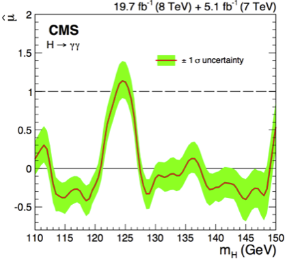
Fig. 82 Best fit of the signal strength \(\hat{\mu}\) as a function of the test mass \(m_H\).

Extracting other parameters

Up to now we have considered only the case where the parameter of interested in our likelihood was the signal strength. Given that all parameters in the likelihood are treated in the same way, we can use the same techniques to extract information about any other parameter. To study the properties of the Higgs boson, we rewrite the signal “\(s\)” as a function of the parameter we are interested in, let’s call it “\(a\)”, and plug \(s(a)\) in the likelihood. Then all we need to do is to rewrite the test statistics as:

\[ q(a) = -2 \ln \frac{L(\mbox{data}|s(a)+b, \hat{\theta}_a)}{L(\mbox{data}|s(\hat{a})+b, \hat{\theta})}. \]

As in the previous definition of the test statistics, the profile likelihood at the numerator is maximized fixing \(a\) and floating \(\hat{\theta}_a\), the value of the nuisance parameters once \(a\) is fixed (i.e. the nuisances are profiled as before), and, at the denominator, the likelihood is maximized against both \(a\) and \(\theta\). As before the 68% and 95% CL interval on \(a\) is evaluated from \(q(a) = 1~(4)\) with all other unconstrained parameters treated as nuisance parameters.
The same idea can be used to scan simultaneously two parameters of interest \(a\) and \(b\). In this case the 68% and 95% CL interval becomes a 2D region such that \(q(a,b) = 2.3~(6)\). It is important to remember that the boundaries of the 2D confidence regions projected on either parameter axis are not necessarily identical to the 1D confidence interval for that parameter, because of the possible correlations between the two (I’m integrating on all the other variables I’m not considering). Examples of 1D and 2D parameter scans are shown in Fig. 83. All the properties of the Higgs boson are extracted from data using this procedure.

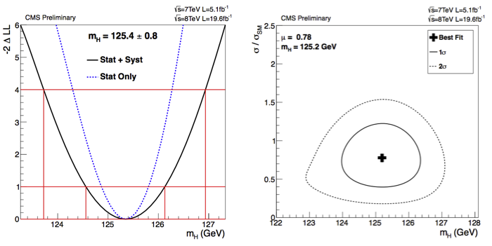
Fig. 83 Examples of parameters scans in 1D (left: \(m_H\)) and 2D (right: \((\mu,m_H)\)).

Bayesian approach to upper limits

The initial Higgs results were indeed verified using both approaches.

The standard prescription to present the LHC results is based on the frequentist paradigma. Nevertheless it is interesting to see how to extract the same results using the bayesian statistics. Using Bayes theorem we can write the posterior for the signal strength as:

\[ f(\mu) = f(\mu|\mbox{data}) = \int\frac{1}{N}L(\mbox{data}|\mu,\vec{\theta})\pi(\vec{\theta})d\vec{\theta} \]

where \(\pi\) is the prior function describing the nuisance parameters and N is a normalization factor to have \(\int f(\mu)d\mu\) =1
The prior presents the usual issues, and it is usually chosen to be flat in the parameter of interest \(\mu\) (assume “total ignorance”). To find the upper limit on \(\mu\) at the \(1-\alpha\) CL (credible level) we need to solve numerically for \(\mu_{1-\alpha}\) in

\[ \int_0^{\mu_{1-\alpha}} f(\mu) d\mu = 1-\alpha \]

see Fig. 84. In general \(\mu\) is a function of the test mass \(\mu = \mu(m_H)\) and to obtain the exclusion plot as in Fig. 81, we will need to compute this integral for each value of the test mass.

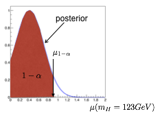
Fig. 84 FIXME Thesis G. Petrucciani.

Look-Elsewhere Effect

Before formalizing the Look-Elsewhere Effect (LEE) for a HEP search, let’s consider this easy example:

Example:

In a city the average number of accidents per day is \(7\pm 1\). When looking at the number of accidents with full moon, the number is 10 which is \(3\sigma\) from the average. Is this sufficient to claim that full moon has an influences on the number of incidents? To answer this question we need to consider the fact that this result was obtained looking at the statistics of this one city. To have a better understanding of the phenomenon we would need to verify it on a larger number of cities. If we repeat the observation on 100 cities, then you would expect that at least one shows a \(3\sigma\) deviation. The question becomes how many cities above 3\(\sigma\) should I observe to convince myself of a supernatural influence of the full moon on the drivers capabilities ?

Back to HEP: consider the search for a resonance in an invariant mass distribution. In case you know that the resonance is expected at \(m = m_0\) (e.g. because you have a theoretical prediction about its position) you can build the discovery test statistics for this fixed mass hypothesis:

\[ t_{\mbox{local}} = -2 \ln \frac{L(0)}{L(\hat{\mu}, m_0)}. \]

Notice that there is no reference to the mass position \(m_0\) at the numerator because we’re considering the case where there is no signal (and so no need to worry about its position). To measure the level of compatibility of your data with the background only hypothesis you can compute the \(p\)-value:

\[ p_{\mbox{local}}=\int_{t_{\mbox{local}}}^\infty f(t_{\mbox{local}} | 0) dt_{\mbox{local}} \]

This is what generally goes under the name of “local” \(p\)-value (often indicated with \(p_0\)).

If instead you don’t know where the peak will appear (a much more frequent situation) the \(p\)-value we are interested in is the one which tells the probability to observe a fluctuation anywhere in the experimentally accessible mass range. The goal is to take care of the trivial fact that with a large enough dataset and a large enough number of bins, we are bound to find a deviation from the background only hypothesis somewhere because of statistical fluctuations. To take this into account the position of the resonance \(m_0\) is replaced by an adjustable parameter in the likelihood:

\[ t_{\mbox{global}} = -2 \ln \frac{L(0)}{L(\hat{\mu}, \hat{m})} \]

the denominator is allowed to fit the strength parameter (\(\hat{\mu}\)) anywhere (\(\hat{m}\)). The corresponding \(p\)-value is:

\[ p_{\mbox{global}}=\int_{t_{\mbox{global}}}^\infty f(t_{\mbox{global}} | 0) dt_{\mbox{global}}. \]

In order to compute this integral, as usual, we need to find the p.d.f. \(f(t_{\mbox{global}} | 0)\). To do this we can proceed brute force tossing toy experiments. This is a particularly computing intensive approach, since we need to scan both the signal strength and the bump position. To overcome this issue it would be tempting to use the asymptotic formulas based on Wald’s theorem we discussed in the previous sections. Unfortunately the Wald’s theorem only works under some “regularity conditions” which require to have the same parameter of interest appearing both in the null and the alternative hypotheses. In our case the alternative hypothesis (denominator) has both the position \(m_0\) of the excess and its signal strength \(\mu\), while the null hypothesis (numerator) has only the signal strength \(\mu = 0\) because the position of the possible excess is not defined in absence of a signal.

A solution to this problem has been developed in [GV10]. The main idea behind the method is to first compute the \(p_{local}\) as if the position of the mass was known and then apply a correction factor to bring it to \(_{global}\):

\[ p_{global} \sim p_{local}+ \langle N(t_{local}) \rangle \]

The factor \(\langle N(t_{local}) \rangle\) is the mean number of times the statistics \(-2\ln L\) cross the \(t_{local}\) threshold from below (slang: “up-crossings”). To understand what this is, let’s take the example of the original paper in Fig. 85

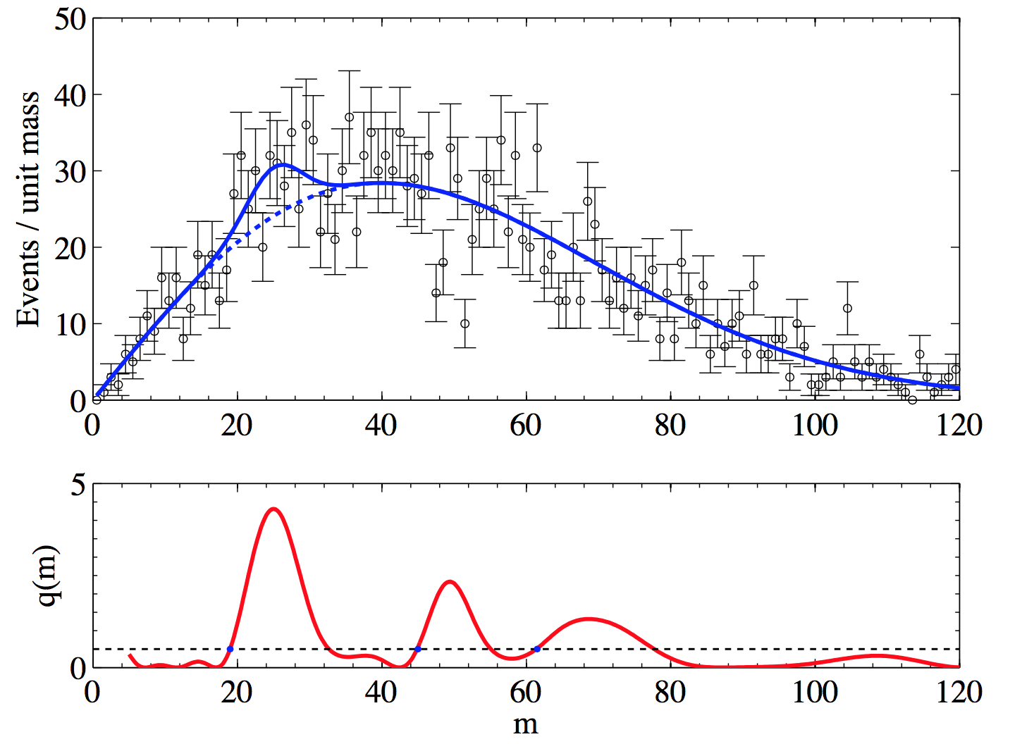
Fig. 85 (top) An example pseudo-experiment with background only. The solid line shows the best signal fit, while the dotted line shows the background fit. (bottom) The likelihood ratio test statistic \(t_{global}\). The dotted line marks the reference level \(t_{local}\) with the up-crossings marked by the dark dots.

The top part of the figure shows a mass spectrum generated on the background only hypothesis. Around 25 there is a hint of an excess, while around 50 and 70 there is an hint of a deficit. The test statistics will be larger the larger the discrepancy of the data from the background only model (the denominator will get the value preferred by the data, while the numerator will adjust the background shape forcing the signal strength to zero). This behavior is clearly visible in the bottom part of the figure, where the three hints of discrepancy manifests themselves as bumps in the test statistics. The procedure would now consist in generating toy experiments and for each of them count how often the \(t_{global}\) test statistics up-cross the value of \(t_{local}\) we observe in data and average this number on the total number of toy-experiments. Up to this point the procedure suffers from the same limitation as the brute force approach to generate toy-experiments to populate the p.d.f. for \(t_{global}\): if we have a large fluctuation in data (remember we’re thinking about a discovery) then \(t_{local}\) is going to be very high and only very few toys will up-cross that high threshold (hence the need of generating a large number of toy experiments). The idea of the paper is that one can compute \(\langle N(t_{local}) \rangle\) for a small value of \(t_{local}\) and then estimate what \(\langle N(t_{local}) \rangle\) would be at any other value of \(t_{local}\) by:

\[ \langle N(t_{local}) \rangle = \langle N(t_{local_0}) \rangle e^{-\frac{(t_{local} - t_{local_0})}{2}} \]

The advantage of this formula is that you can compute \(\langle N(t_{local}) \rangle\) with a very small number of toy-experiments and then propagate the result.

The example treated in this section refers to the most common case of the search of a resonance appearing as an excess in a mass distribution. The same ideas obviously can be applied to any other search where instead of a bump in a mass spectrum the deviation from the background only hypothesis appears in another variable or in a more general case in a set of variables (e.g. search for an excess where you don’t know neither the position nor the width).

References

Most of the material of this section is taken from:

• R. Barlow, [Bar89], “ A guide to the use of statistical methods in the physical sciences”. Ch. 7

• G. Feldman and R. Cousins, [FC98], “Unified approach to the classical statistical analysis of small signals.”

• A. L. Read, [Rea00], “Modified frequentist analysis in search results (CLs method)”

• G. Cowan, K. Cranmer, E. Gross, O. Vitells, [CCGV11], “Asymptotic formulae for likelihood-based tests of new physics”

• E. Gross and O. Vitells, [GV10], “Trial factors for the look elsewhere effect in high energy physics”